Muon Decay in the MINERvA Experiment
Margaret Menzies – Harbor City International School, Duluth, MN
Jackie Kitchenhoff - Northland High School, Remer, MN
Dr. Richard Gran - University of Minnesota Duluth, Duluth, MN
Students use actual MINERvA detector event data to find and record decay events from a particle called a muon, understand how atomic and subatomic decay processes work by seeing them happen. They calculate the average lifetime and half-life for the muon and also study conservation of energy
Conservation Laws of Collisions
(Billiard Ball Collisions on the Particle Scale)
Paul Conrow – Rochester City School District, Rochester, NY
Carol Hoffman – Hilton Central School District, Hilton, NY
Jeffrey Paradis – Rush-Henrietta Central School District, Henrietta, NY
Paul Sedita - Canandaigua City Schools, Canandaigua, NY
Dr. Kevin McFarland – University of Rochester, Rochester, NY
Students use actual MINERvA detector event data to find and record particle collision events between a neutrino and neutron (within the nucleus), understand how conservation of momentum and energy on the particle scale. Calculations made will help determine the original momentum and kinetic energy of the incoming neutrino.
Editing, Technical Work
Dr. Nathaniel Tagg– Otterbein University, Westerville, OH
Rev. July 2015
You will find all of the materials listed below (and additional PowerPoint presentations) on the web page: http://neutrino-classroom.org
Particle Physics Activities for High School Physics Students
Why do you want MINERvA in your curriculum?
The essential questions you can explore with this material
Technical details on the Arachne program
Particle Pre-Assessment for Students
Activity: Radioactive Decay of M&M’s
Activity: Modeling Radioactive Decay with Dice
Activity: Finding Muon Decays with MINERvA
Identifying Decay (Michel) Electrons with Arachne
Activity: Measuring the Muon Lifetime
Activity: Build a Model of MINERvA
Activity: Conservation of Momentum when Neutrinos Interact
Activity: Neutrino Scattering and the Target Nucleus
Standard Model Poster Scavenger Hunt
Additional background information
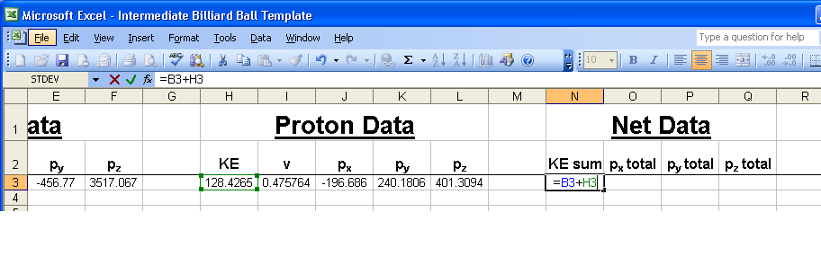
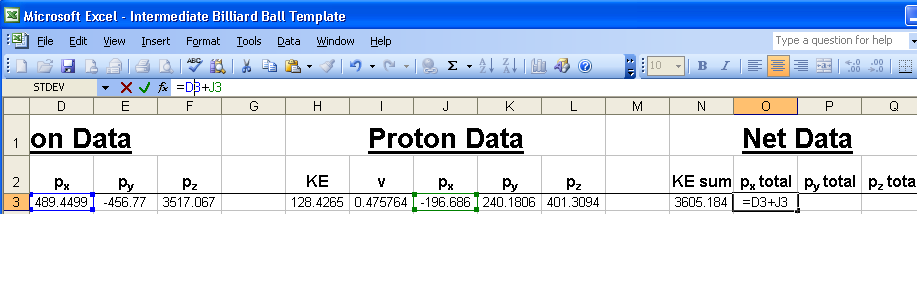
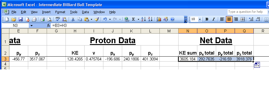
Merging Excel Spreadsheets from Student Groups
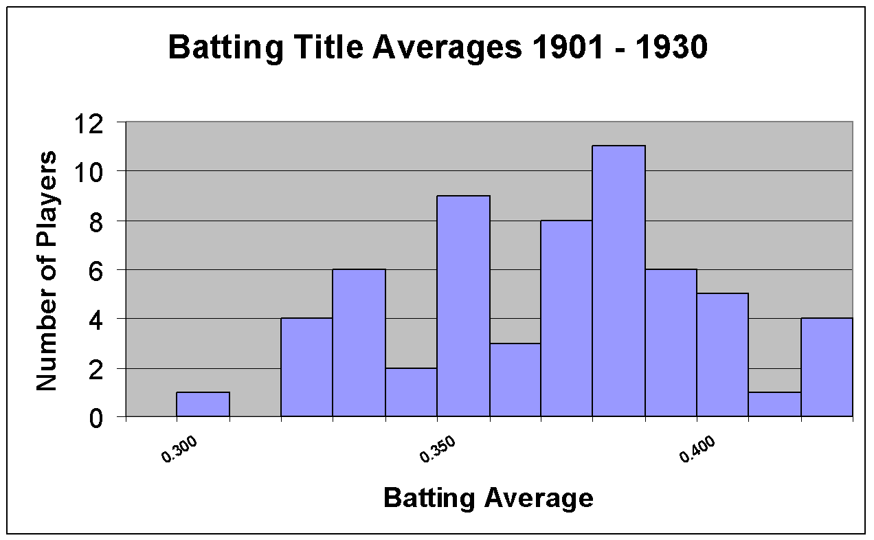
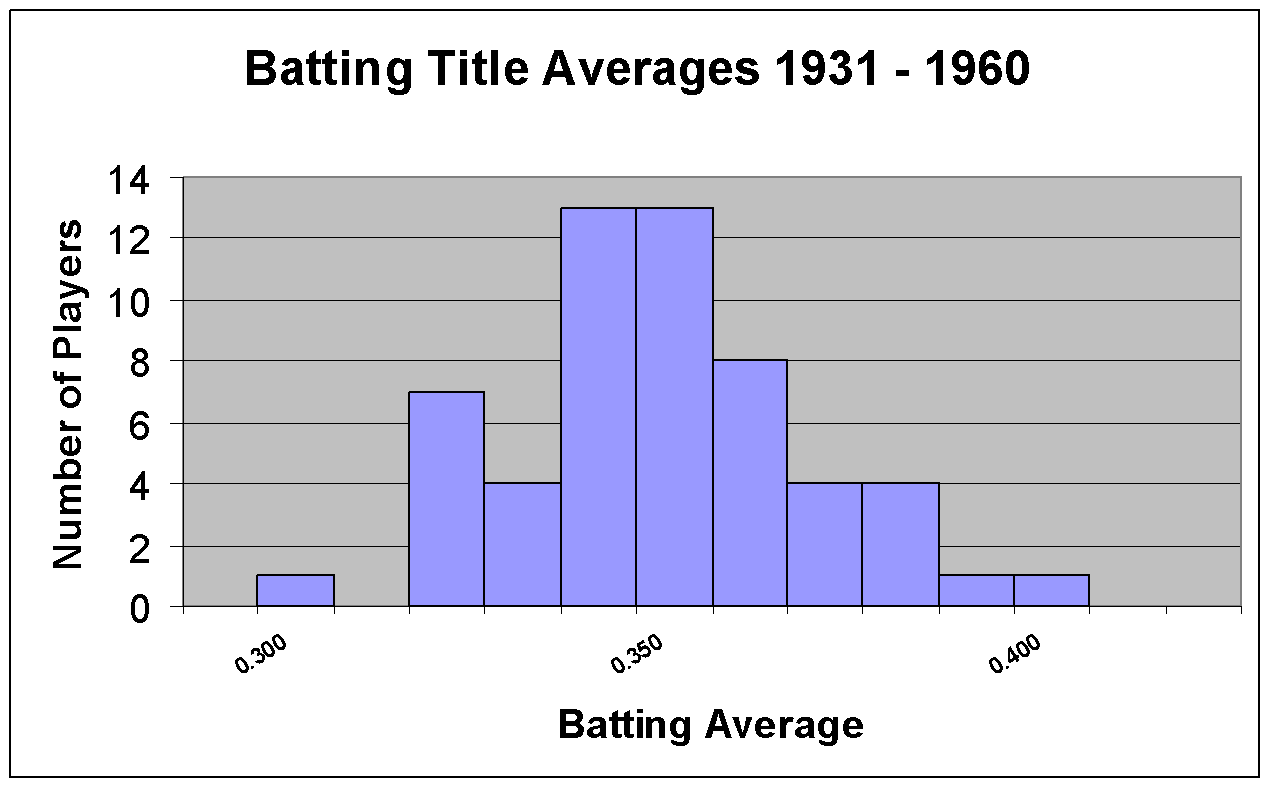
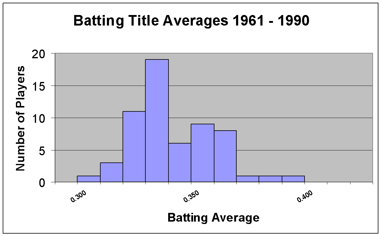
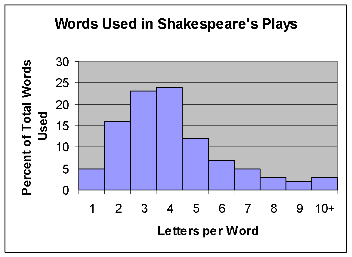
Teacher background Information for Introducing Histograms to Students
Explore cutting edge science in the fascinating world of particle physics.
Students use real particle physics data to explore two standard physics topics
1. Radioactive decay: the random process and lifetime of a particle called a muon.
2. Measuring conservation of momentum and energy when particles collide.
Insight into how practicing scientists creatively solve problems and explore the unseen world of fundamental particles
You don't have to be Einstein to get involved with particle physics.
Choose as much or as little as you like to add depth to your physics curriculum, or offer parts as an optional activity for students or an after school science club.
Arachne is named after a character from mythology who lost a weaving contest to MINERvA. The Arachne program was created in order to visualize particles that were recorded by the MINERvA detector. It pulls calibrated data from a server at Fermilab and then draws a few pictures and graphs to summarize what happened in the detector.
Arachne requires a recent version of a web browser, such as Firefox version 4.0, Safari version 4.0, and Chrome version 5.0. Arachne relies on Java and parts of the HTML5 standard to more dynamically render the images and make them interactive. Because it does not yet support the latter, the Internet Explorer browser will not run Arachne.
The day before your class, be sure to check that the server is responding. It occasionally goes down.
There are a number of interesting things so see in the MINERvA data, but we have chosen two different threads that illustrate and reinforce ideas that are already part of your physics and chemistry curriculum.
Muon Decay is an example of radioactive decay. In chemistry or physics class, the concept seems abstract, something that happens unseen inside lumps of material like uranium or aging trees. These activities let you observe real decays and measure their decay time one-by-one, in the comfort of your own classroom.
In the MINERvA detector particles with charge produce visible tracks that can be followed, which is what this activity is all about, using real-event data showing muon decay to Michel electrons. They are named for Louis Michel (1923-1999), the French physicist who provided the first documentation of the decay sequence of muons to an electron and two neutrinos: A development not so different from Marie Curie's pioneering initial work on radioactive decay. MINERvA is capable of detecting an array of events. We will be focused on muon decay events in these activities, but students are likely to observe other events if they do any exploring of data on their own. (Arachne Scavenger Hunt) Further background on the types of events detected in MINERvA is outlined in a PowerPoint presentation on Types of Events.
Billiard Ball Collisions involving conservation of momentum and energy, is a familiar introductory physics topic. The same conservation principles and visualization applies to particle interactions, too. The simplest examples even look like the collision of two billiard balls, but also reveal something of the inner workings of the atomic nucleus.
Below, we suggest a sequence of activities for each topic. Depending on your class, schedule, or other considerations, you can shorten the activities, or in some cases assign pieces as homework instead of doing them in class.
Muon Decay Activities
Introductory Activities - (I) Data Analysis- (DA) Enrichment Activities - (E)
Prior Knowledge Activities:
(I) Particle Pre-Assessment for Students
(I) Particle Adventure1
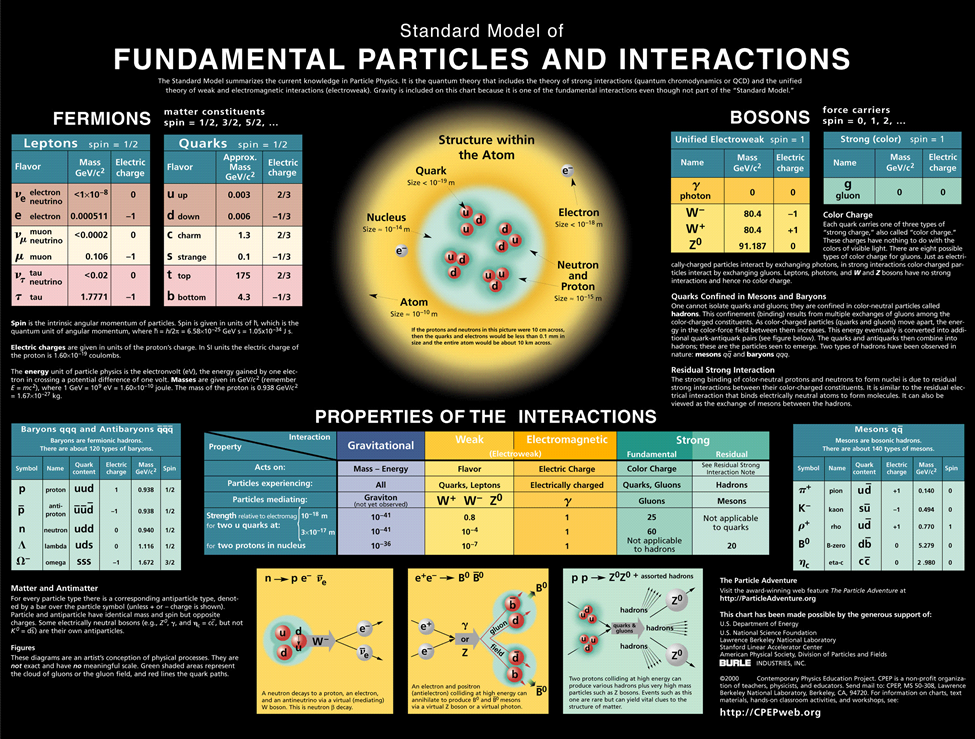
(I) Standard Model Poster scavenger hunt
(DA) Histogram Activities3
Classroom Activities:
(I) Activity: Modeling radioactive decay with dice (60 minutes)
(I) Activity: Radioactive Decay of M&M’s
(I) What is MINERvA? – PowerPoint (20 minutes)
(I) Directions for Simple Arachne (Arachne basics for muon decay) - Tutorial (20 minutes)
(I) Activity: finding muon decays with MINERvA- teacher guided (30 minutes)
(I) History of the Neutrino “Norton Nabs a Nu” – PowerPoint (30 minutes)
(E) Types of Events – PowerPoint (30 minutes)
(DA) Activity: Measuring the muon lifetime (90 minutes), data analysis, calculations and
graphing data (180 minutes),
Optional/Extension Activities:
(E) Arachne Scavenger Hunt
(DA) Neutrino Birth and Death PowerPoint
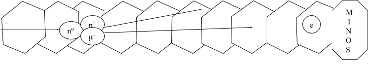
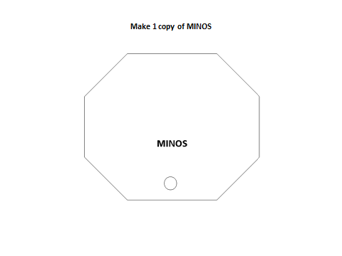
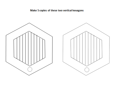
(I) Activity: Build a model of MINERvA
(E) Activity: Energy of Decay electrons (Understanding why the electrons in muon decay have this distribution of energy)
(I) Particle Events in 60 seconds
(I) See what the MINERvA detector is doing right now
(E) Neutrinos in 60 seconds
(E) Kevin McFarland’s neutrino talk for students
Billiard Ball Collisions (Conservation Laws) on the Particle Scale
Introductory Activities - (I) Data Analysis- (DA) Enrichment Activities - (E)
Prior Knowledge Activities:
(I) Particle Pre-Assessment for Students
(I) Particle Adventure1
(I) Standard Model Poster scavenger hunt
(DA) Histogram Activities2
Classroom Activities:
(I) History of particle physics and MINERvA – PowerPoint (30 minutes)
(I) What is MINERvA? – PowerPoint (30 minutes)
(I) Directions to Simple Arachne – Tutorial (30 minutes)
(I) Bug and Truck Collision – PowerPoint (30 minutes)
(I) Activity: Conservation of momentum when neutrinos interact– teacher guided (60 minutes)
(I) Ten collision sampler (30 minutes)
(I) MINERvA Momentum Model – PowerPoint (30 minutes)
(I) History of the Neutrino “Norton Nabs a Nu” – PowerPoint (30 minutes)
(DA) Activity: Neutrino scattering and the target nucleus (60 minutes), Continue data analysis
Optional/Extension Activities:
(E) Arachne Scavenger Hunt
(DA) Neutrino Birth and Death PowerPoint
(I) Activity: Build a model of MINERvA
(I) See what the MINERvA detector is doing right now
(E) Neutrinos in 60 seconds
(E) Kevin McFarland’s neutrino talk for students
1 - Particle Adventure is an excellent online resource that provides a fairly quick introduction to particle physics and fundamental particles. It was produced and is maintained by the Particle Group of the Lawrence Berkeley National Laboratory. Here is the website: http://www.particleadventure.org/index.html. Once at the website, choose “The Standard Model” option. This is divided into four major parts. For a good unit introduction we suggest using “What is fundamental?”, and “What is the world made of?” “What holds it together?” follows these first two and should be considered optional as it provides background on fundamental forces and their interactions which is not critical to this unit's focus. “Particle decays and annihilations” follows this section and should be used with students to provide some overview of decay
2 - Histogram activities are provided if you think your students could use further background in the purposes, construction and appropriate uses of histograms for scientific data.
Goal
A quick assessment for teachers to use to gauge the content that students already have in the topic of modern physics.
Notes for the Teacher
Each student enters physics with a different set of knowledge. This questionnaire is meant for the students to take so that the teacher can determine what Prior Knowledge Activities might be appropriate so that the students feel more comfortable heading into the unit.
Student Instructions and Worksheet
Particle Physics Pre-Assessment
Directions: Answer each of the following questions with honesty and thorough thought. The answers that you give are going to help your teacher structure your particle physics unit.
Very Comfortable | Comfortable | Barely Comfortable | Not Very Comfortable |
_______ Wikipedia _______ other websites | _______textbooks _______ textbook extras | ________ other students ________ other |
Goal
This simulation provides a simple example of the rate at which a radioactive isotope decays.
Materials
M&M™ candy pieces
resealable bag
graph paper
Teacher's Notes
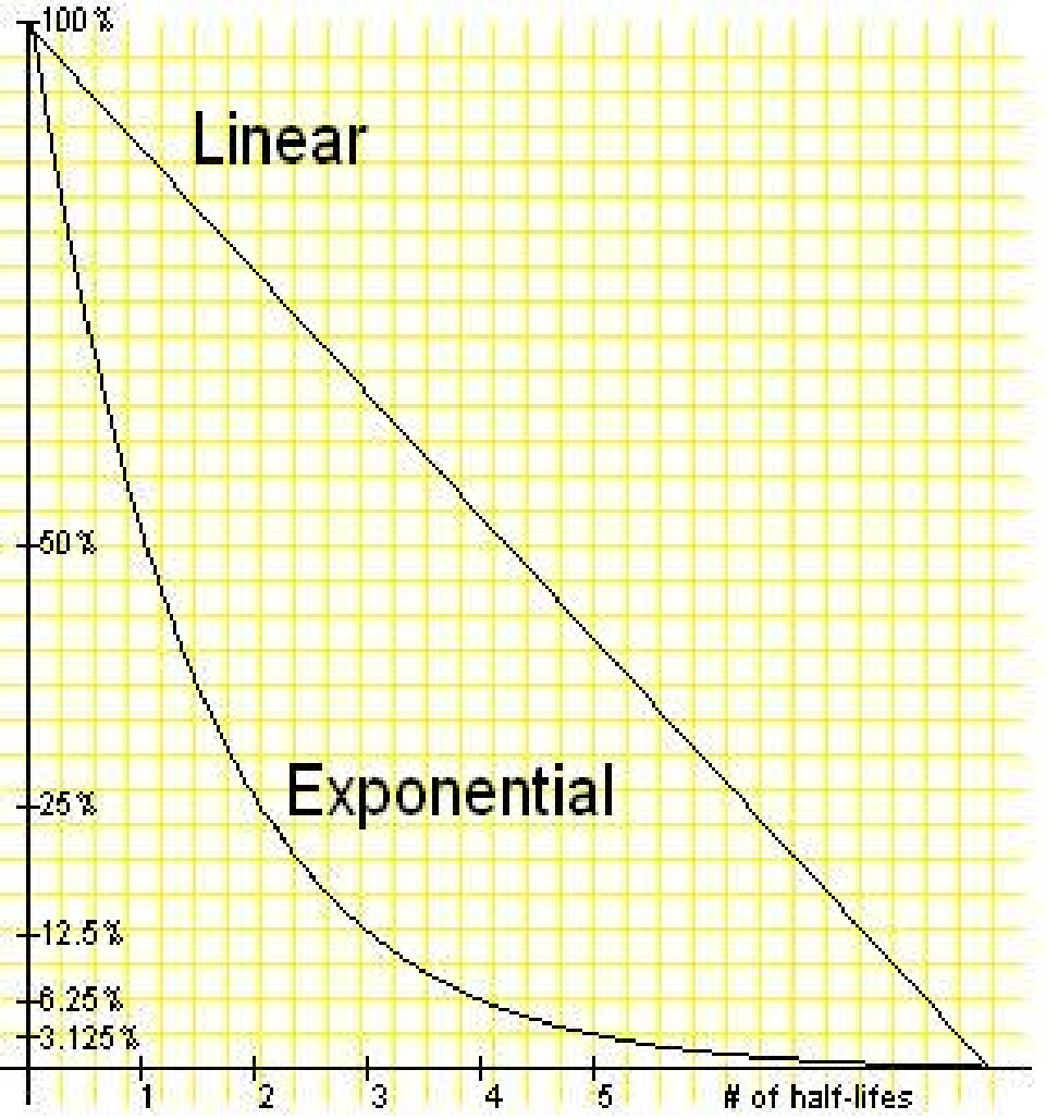
Some naturally occurring isotopes of elements are not stable. They slowly decompose by discarding part of the nucleus. The isotope is said to be radioactive. This nuclear decomposition is called nuclear decay. The length of time required for half of the isotope to decay is the substance's half-life. Each radioactive isotope has its own particular half-life. However, when the amount of remaining isotope is plotted against time, the resulting curve for every radioisotope has the same general shape.
Hint: Make sure you use candies with printing on one side (plain M&Ms™).
Answers to Extensions
Half-life is the length of time required for one half of an isotope to decay.
The half-life of M&Ms™ in this activity was 10 seconds.
At the end of two half-lives, 1/4 of the original sample remained and 3/4 of the sample had decayed into a new element.
The graph is a decreasing logarithmic curve.
The shape of the graphs will be almost the same.
The shape of the graphs will be almost the same.
Student Instructions and activity sheet
Procedure
Place 50 atoms (M&Ms™) in the bag.
Seal the bag and gently shake for 10 seconds.
Gently pour out candy.
Count the number of pieces with the print side up—and record the data. These atoms have "decayed".
Return only the pieces with the print side down to the bag. Reseal the bag.
Consume the "decayed atoms”.
Gently shake the sealed bag for 10 seconds.
Continue shaking, counting, and consuming until all the atoms have decayed.
Graph the number of undecayed atoms vs. time.
Data and Observations
Half-life | Total Time | # of Undecayed Atoms | # of Decayed Atoms |
0 |
|
|
|
1 |
|
|
|
2 |
|
|
|
3 |
|
|
|
4 |
|
|
|
5 |
|
|
|
6 |
|
|
|
7 |
|
|
|
8 |
|
|
|
Questions
What is a half-life?
In the experiment, what was the half-life of the M&Ms™?
At the end of two half-lives, what fraction of the atoms had not decayed?
Describe the shape of the curve drawn in step 9.
Repeat the experiment three more times, starting with 30 atoms, 80 atoms, and 100 atoms of ‘candium’. Compare the resulting graphs.
Repeat the experiment using half-lives of 5 seconds, 20 seconds, and 1 minute. Compare the resulting graphs.
(Arachne basics for muon decay)
Goal:
The information below should be reviewed by both the teacher and the students so that everyone has a basic knowledge of how the Arachne site works and relays data
http://minerva05.fnal.gov/Arachne/simple.html
DATA:
[Analogy: the Run is like a roll of film…the Entry (Gate) is each individual picture on the film… the Slice contains the details within each picture]
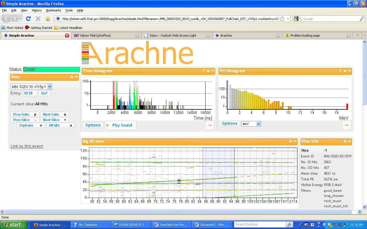
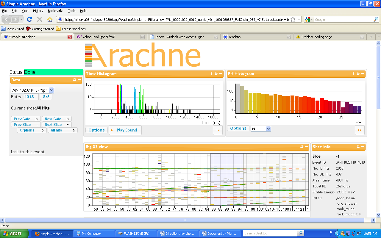
TIME HISTOGRAM:
PH HISTOGRAM:
BIG XZ VIEW:
MAGNIFIER WINDOW:
MAGNIFIER WINDOW:
HIT MAPS:
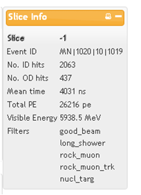
SLICE INFO:
3D DISPLAY:
dimensional view of the
particles’ paths through the
detector
This is the first activity in learning about radioactive decay
Goals
1. Start with a physical, tactile simulation of radioactive decay.
2. See the exponential and random nature of a decay process directly.
3. Play dice with the Universe.
Radioactive decay, as it is often taught, is abstract. We talk about piles of radioactive material, a “decaying exponential” mathematical function, and how it is dangerous, but these things are happening at an atomic level we can't actually see or experience with our hands or eyes directly. The two variations here let us do that, making clear both the intrinsically random, but at the same time the intrinsically exponential nature of the process. Then in muon decay activity two, with data from MINERvA, we will take an actual decay process which is also usually unseen, and make it visible too.
Prior Knowledge:
Examples of radioactive decay from the news or elsewhere, such as carbon-14, the M&Ms™ lab, medical tracer isotopes, or the storage of nuclear waste.
Materials:
Dice
Paper to record the data, graph paper to make a histogram
Calculator
Notes for the teacher
What is radioactive decay, and what other things in nature share the same characteristics? The process of radioactive decay, of atomic isotopes or fundamental particles, is intrinsic to the universe and to particle physics. The mathematically characteristic exponential decay (and the related exponential growth) is found in lots of places in nature; anywhere the rate of change of something is proportional to the amount of that something. Radioactive isotopes, bacteria populations, investments in a bank account. The other characteristic of radioactive decay is its inherent randomness, which is pretty astounding by itself, and is a core feature of quantum mechanical systems. The random nature also leads to some interesting issues in observing and measuring the decay, problems shared with other inherently random things such as political polling and the ubiquitous ±3% error and separately with rolling dice. These activities use the dice process to give you a tactile, physical experience with what is really happening in these other processes that are nanoscopic or abstract.
There are two related pieces here. Rolling one hundred dice several times, and rolling a single die multiple times, then repeating that a hundred times. Here, we've assumed you are able to do both, possibly saving the second one as an out-of-lab homework activity. It is reasonable that, due to time or material constraints, you choose to do only the second one or only the first. If you picked this up with the MINERvA muon decay activities, the second one is the most like what the students will experience looking at muon decay.
The two ways are first summarized here, together. The student instructions break them into two separate, with specific instructions and questions for the group doing the activities.
First way: roll one hundred dice (multiple times) to represent a sample of a hundred radioactive isotopes decaying over time. This does a good job of illustrating the idea of "half-life" and the exponential decrease in the activity of a radioactive sample over time. The question you are asking is “how many remain after some time”. Such samples might be medical isotopes, waste from your local nuclear reactor, or the uranium and thorium atoms that remain on earth long after they were formed ten billion years ago in supernovae.
Second way: roll a single die (multiple times) to represent how long a single muon lives, then do it again for the next muon, and the next, one hundred times. This is a good way to illustrate the range of lifetimes you will observe if you have a sample of unstable particles such as muons. The question you are quantifying is “how long (what range of times) does each particle live”. Such samples are common in particle and nuclear physics.
In fact, these two illustrations are just two ways of looking at the same phenomena. After doing one or both activities, it should be clear that you are observing a random process, observing many at once, or one at a time doesn't matter, and they both lead to the exponential decay that is characteristic of the random process. This will also help overcome the problem that you can't “see” radioactive isotopes or muons; it makes these real but hidden details plain. As a bonus, you will also observe how the randomness also means you will get somewhat different results when you repeat a measurement with otherwise identical initial conditions, such as you might have noticed applies to political polling, and maybe baseball, among other everyday phenomena.
Doing the second variation only: If you are not able to obtain enough dice, you can do the second activity only. And anyway, the second variation better matches the muon decay activities involving the MINERvA data. When you prepare the instructions for students, trim out the references to the first variation.
Doing the second variation as homework: If you think it is likely that your students have at least one board game at home with dice, you can assign the second activity (which takes more time) as homework, and have each student bring their results in for discussion and be ready for the muon data.
Using spreadsheets or other software: This exercise is designed to be done with paper and pencil and calculator, but for students who are prepared, interested, and want to, you can use computer software such as Excel or more advanced software like Matlab, to explore things more quantitatively. We recommend you press on quicker to get to the muon decays in the MINERvA data, but you might know just the student who wants something more advanced.
Instructions for students
What is radioactive decay, and what other things in nature share the same characteristics? The process of radioactive decay, of atomic isotopes or fundamental particles, is intrinsic to the universe and to particle physics. The mathematically characteristic exponential decay (and the related exponential growth) is found in lots of places in nature; anywhere the rate of change of something is proportional to the amount of that something: radioactive isotopes, bacteria populations, investments in a bank account. The other characteristic of radioactive decay is its inherent randomness, which is pretty astounding by itself, and is a core feature of quantum mechanical systems. The random nature also leads to some interesting issues in observing and measuring the decay, problems shared with other inherently random things such as political polling and its ubiquitous ±3% error and separately with rolling dice. These activities use the dice process to give you a tactile, physical experience with what is really happening in these other processes that are nanoscopic or abstract.
First way: one hundred at once.
You need: a large supply of dice (about one hundred), a cup or bucket large enough for them, a sheet of paper to record data, and some graph paper for graphing your results.
Imagine: you have a supply of some radioactive isotope that has a 1/6 chance of decaying in the next minute. How much of that isotope remains after six minutes? How about after 20 minutes? How much time does it take for approximately half the sample to decay?
Put all the dice in your cup or jar and roll them on the table.
Separate all the dice that turned up “1”, these are the particles that decayed.
Count and record those that decayed and those that remain, measured after “one minute” passed.
Separate the decayed “ones” into a pile that you can see later, while you roll the non-ones again.
Consider: is the pile of decayed dice about as many as you expect? Was it exactly as many as you expected?
Put the others (the ones showing 2-6) back into the cup.
Repeat all these steps and record a measurement of what decayed during and what remains after two minutes. Separate this next batch of dice that turned up “1” into its own pile next to the first – you will save the progression of decays so you can see the process visually, in addition to the numbers you have recorded.
Repeat again for the third minute.
Repeat again and again until they are all decayed.
You now have a sequence of piles you can see (and numbers recorded that you can graph) that represent how many decays happened during each minute. Describe you can see both these seemingly contradictory properties: a) the number of decays is proportional to the number available to decay and b) the number that decayed is random.
Let’s represent the situation with a couple graphs. Graph the number that decayed in each minute, using a histogram or bar chart. Separately, graph the number that remain undecayed in the sample, using a histogram or bar chart.
Estimate from your graph, by counting, how much time it takes for approximately half the sample to decay. Draw a mark or an arrow on the horizontal axis of each graph indicating where this time is.
Look up the exponential decay function; if you have a graphing calculator or similar program, plot it with a constant of (0.16666666 = 1/6), in other words, plot with its negative sign: e-(1/6)x . If you have a regular calculator, compute ten or so values and make another graph of it on your paper. Does that function describe the data you graphed? If you have access to the right software, you might even be able to plot your data and ask the software to fit an exponential, but sketching this one by hand would be good enough. Does the inherent randomness of this process make it difficult to see the exponential nature, and if so, can you think of a change in your procedure
How do you feel about the idea that there was likely a die that remained and didn't decay for fifteen to twenty rolls? Is it possible that one could remain for a hundred or more rolls?
Second way: simulating one hundred separate muons
You need: one (or a few) dice, a bit of time, a few pieces of paper for recording your data, and a couple more for graphing.
Imagine: you are creating, and then observing an unstable particle like a muon or a neutron, and can measure how long each one of them lives, one by one. Each one has a 1/6 chance of decaying in the next one nanosecond, you will count the number of nanoseconds until each one decays. Do you expect short lifetimes to be more common, or long lifetimes, or something in the middle? What is the longest you expect to see a particle live? Can you guess what the average (mean) lifetime will be, when you are done and have analyzed all the decays?
Take your die and count the number of rolls until you roll a “1”, and record it on your piece of paper.
Repeat about 100 times, each time recording the number of rolls until you roll the number “1”. You have some quality time during this activity to consider the questions mentioned in the “imagine” paragraph above, and what you learned from activity one. (You could divide the effort among three or four people and get it done in 1/3 or 1/4 the amount of time, if you are in a hurry.)
Let’s graph the results. Look at the data, and count the number of times where the muon lasted up to one nanosecond. Record that on a graph in the 0-1 interval. Count the number of times it took two rolls, and record that in the 1-2 interval. You are making a histogram of the decay time. Continue until you have filled all the intervals; toward the end many of them will be filled with zeros, with occasional intervals where a few long-lived particles fall.
Now compute the average life, in nanoseconds. Clearly you can average all 100 numbers you recorded by adding them and dividing by 100. You might see that you can do this more quickly from your graph than you can from the sheet with 100 numbers on it, but either way works. Draw a mark on the horizontal axis of your graph to represent the average lifetime.
Look up the exponential decay function; if you have a graphing calculator or similar program, plot it with a constant of (0.16666666 = 1/6), in other words, plot with the negative sign: e-(1/6)x . Does that function describe the data you graphed?
Does the inherent randomness of this process make it difficult to see the exponential nature, and where is it the most difficult? Why?
How do you feel about the idea that there was likely a muon that remained and didn't decay for fifteen to twenty rolls? Is it possible that one could remain for a hundred or more rolls?
Now what are your answers to these questions: do you expect short lifetimes to be more common, or long lifetimes, or something in the middle? What is the longest you expect to see a particle live?
If you have done both exercises, your one graph from the second exercise is most like which graph from the first exercise? And it should look approximately like the other graph from the first exercise, but 6 times smaller. In these cases, they should look similar enough that you can recognize the similarity, but they certainly won't be identical.
How would you explain why they should look so similar but not identical?
What would happen if you repeated one or the other exercise again, would the results be identical? For both exercises, you had one die that lasted the longest, but might you ever expect to see a particle last ten-times that long? What would happen if you had the luxury of doing 1,000 trials, or 1,000,000 trials, or an Avogadro’s number (6.02 x 10²³) number of trials?
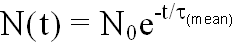
The function that best describes these graphs is a decaying exponential Ne-t/τ, (sometimes also written Ne-λt ) where our situation is such that t is time, N is either the initial number of particles that might decay, or the initial activity which is 1/6 of the number of particles, and τ (tau) is the mean lifetime which is 6 seconds or nanoseconds depending on which activity you are doing or λ which is the probability that a particle will decay in the next bit of time. This function occurs a lot for interesting random and non-random situations, but random processes often give rise to behavior that can be described mathematically like this.
Notice, in the second activity you directly measured the value of this parameter τ tau = mean lifetime. If you recognized how the second activity is the same as the first, then you have again measured it. Go back to your first data set and calculate the mean lifetime there. Is it the same? Should it be? What is the accuracy of your measurement and the role of random fluctuations in your measurement? If you had a need to make a more accurate measurement, how would you do it?
Advanced questions:
You might notice that the spot where you marked “half-life” in the first activity is not at all in the same location as the spot you marked “mean-life” in the second activity. These are different. Think carefully about how you knew where to mark those spots and try to describe the subtle difference between them.
Political polling has been mentioned as another random process that we suppose you have encountered. Though it doesn't obviously give rise to an exponential distribution, but it clearly does give rise to fluctuations between repeated measurements of apparently the same thing, such as the public's support one or the other political candidate. If you don't expect two polling firms to get the same answer if they poll on the same night, how can you still draw conclusions from their results?
I teased that the same issues involving random processes might also apply to the game baseball. Think on that.
If you are comfortable enough with your calculus, you can derive the connection between the probability to decay and the exponential function. An internet search or textbook will get you started.
If you are comfortable enough with programming, and can find a pseudo-random number generator to use, you can explore further and faster than you can with dice. Using the same 1/6 probability, code the procedure into a program. Use a programming platform like C++, Java, Matlab, Mathematica, or possibly even a spreadsheet. When it's ready, play with the mean lifetime and compare the exponential to high statistics histograms. Then play with changing the time step or probability.
This is the suggested second activity for learning about radioactive decay. It is suggested that this be a teacher guided activity.
Goals
To observe and analyze specific examples of a particular radioactive decay process: muon decay.
Practice taking data for the main activity to quantify the nature of decay times.
Reinforce the randomness inherent in the decay process.
Prior knowledge
Know a few fundamental particles: muons, electrons, neutrinos.
Know the basics of radioactive decay (from the dice activity or elsewhere)
Have an understanding of the MINERvA experiment and the structure of the detector.
Materials
Website access to Arachne (Firefox, Chrome, Safari, not Internet Explorer see note)
Practice run data sheet handout for ten events.
Follow-up questions handout.
Notes for the teacher
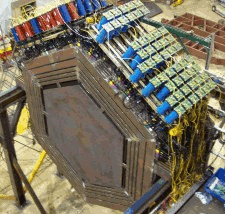
The MINERvA detector and what it records. Depending on the order in which you have chosen to do the material in this packet, this is the first use of MINERvA data for you. In brief, MINERvA is a detector located in a neutrino beamline at Fermilab, near Chicago. As is typical of a particle detector, MINERvA only records the passage of charged particles; neutral particles (neutrinos, neutrons, and photons) are invisible until they interact with an atomic nucleus in the detector and transform into or produce new charged particles. The main view of these interactions is the XZ view, which is the top view of the activity in the detector, and you can see things travel from front to back, left to right. Many charged particles, especially muons, look like simple and long “tracks” of activity left behind as the particle passed through. Some particles, especially electrons, look like little splashes of activity that are well localized and may be made of only a few hits. We have another activity [link to it] with material that gives a broader background to the detector and what it was designed for.
Muon decay: If you did the dice activity, or other activity, you are familiar with the basics of radioactive decay. A particle or nucleus spontaneously (and randomly) changes into one or more new particles (or a new nucleus and some particles). The resulting state is energetically favorable, so there is always additional energy available to become kinetic energy. Specifically, the muon decays similar to the classic “beta decay” (similar to carbon-14 and also like neutron decay) giving an electron and two neutrinos as products. If you are familiar with the standard model of particles, muons are a heavy cousin to the electron; the technical term for this family of particles is leptons. So the muon decays into its less massive lepton cousin. The neutrinos are neutral, so they are usually unseen as they escape the point of the decay, so the signature is a muon stopping in the detector then the electron from the decay appearing. We can write this reaction in a form similar to how we right chemical reactions
μ- → e- + anti-ve + vμ
muon decays to electron, anti-electron neutrino and muon neutrino
Particle interactions and conservation laws: This is a good place to look at rules for particle interactions. Notice first that the charge stays the same on both sides of the decay, so charge is conserved. Both the muon and the electron are in the lepton family, but particle physicists say they have different “flavor”, muon flavor and electron flavor. Notice then that there is still one of each flavor on the right side after the decay has happened. In fact, we have carefully written that there is an electron and an electron anti-neutrino, a particle and anti-particle pair, so the left side has no electron-ness at all while the right side the electron-ness cancels out or sums to zero, like adding a +1 and a -1 together. This chemical reaction style statement doesn't say so, but of course momentum and energy were conserved. The muons you will see came to rest with no kinetic energy and no momentum. For momentum to be conserved, neutrinos must have come out in roughly the opposite direction to the electron (but we won't see them). For energy to be conserved, the rest energy (mass) of the muon, 107 MeV, was converted according to E=mc2 into the kinetic energy of the three products, some of which was given to the electron which we measured; half or less goes to the electron.
Measuring Muon Decay- Initial Ten Practice Run Data Sheet
# | Event ID | Slice Number | Mean Time (ns) | Visible Energy (MeV) | Time Difference = #2 Mean time minus #1 Mean time | Notes and Questions |
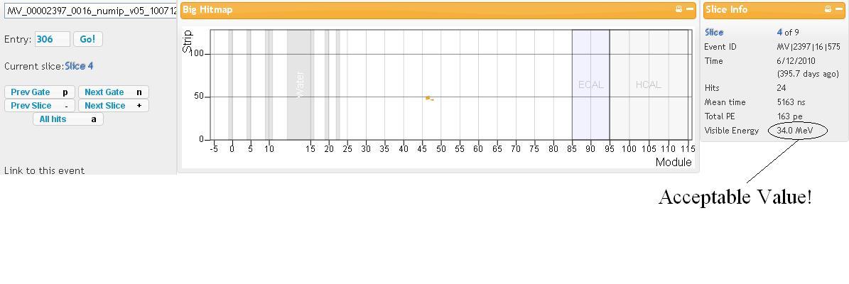
1 | MV 2397/16/575 | 1 | 2385 ns | Example | ||
2 | 4 | 5136 ns | 34.0 MeV | 5136-2385 = 2751 ns | ||
1 | MV 2397/16/631 | 4 | 6069 ns | |||
2 | 6 | 7340 ns | 40.1 MeV | 1271 ns | ||
1 | MV 2397/16/845 | 2 | 4010 ns | |||
2 | 8 | 9339 ns | 24.3 MeV | 5329 ns | ||
1 | MV 2397/16/871 | 2 | 8823 ns | |||
2 | 4 | 10489 ns | 20.3 MeV | 1666 ns | ||
1 | MV 2397/16/921 | 4 | 4287 ns | |||
2 | 7 | 11164 ns | 30.4 MeV | 6877 ns | ||
1 | MV 2397/16/1244 | 3 | 4357 ns | |||
2 | 4 | 5840 ns | 25.3 MeV | 1483 ns | ||
1 | MV 2397/16/1453 | 2 | 4042 ns | |||
2 | 4 | 5117 ns | 58.9 MeV | 1075 ns | ||
1 | MV 2397/17/287 | 1 | 2462 ns | |||
2 | 7 | 6068 ns | 29.0 MeV | 1174 ns | ||
1 | MV 2397/17/903 | 6 | 7641 ns | |||
2 | 7 | 8770 ns | 15.0 MeV | 1129 ns | ||
1 | MV 2397/17/959 | 6 | 7779 ns | |||
2 | 8 | 10456 ns | 33.5 MeV | 2677 ns |
Other tips on this activity or questions that may come up:
Where do the muons come from, if this data is from a neutrino beam? Most of these muons were one of the neutrinos, before it interacted in the rock in front of the detector. After it changed from a muon neutrino into a muon it travelled out of the rock, through the air a bit, and into the front of the MINERvA. You can see other neutrinos interacting in the MINERvA detector itself (not in the rock) too, as you look through the data for muons and their decay.
Answers to the follow-up questions
1. As you flip through the time-slices of Muon Decay Event One, how many have activity that is track-like? How many are small splashes of energy?
Two slices have tracks, four slices have splashes, one slice has both (though there may be different interpretations of whether these shorter ones are tracks or splashes) and two slices that have nothing.
2. There were actually two time-slices in Event One, each with a small splash, that occurred at the end of the muon track. How did you know which one was the decay electron and which one to reject as some other unrelated thing?
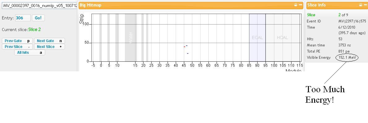
The splash in slice two had energy that was too high, 152.1 MeV, which is well over the expected range of 60 MeV or less. It is just a coincidence that something else happened in the right location.
3. Considering all eleven links, which one has the most time between the decay electron and its parent particle? Which one has the least time?
Event five = MV/2397/16/921 has the highest at 6877 ns.
Event seven = MV/2397/16/1453 has the lowest with 1075 ns.
4. In addition to all the muons that stopped in the middle and decayed, what was the most interesting other thing you saw?
A variety of answers are possible, though there is a neutrino interaction in the same link as seven in MV/2397/16/1453 that we think stands out as interesting.
5. The muon you find is always traveling left to right, then stopping somewhere in the middle. How about the electrons?
Since the muon is at rest when the decay happens, the electron can go in any direction it chooses (it chooses randomly), so it may or may not move in the same direction as the muon travelled. In these ten decays you see all the variations. In contrast, if the muon was moving (its not), then to conserve momentum, the decay electron would probably be moving in roughly the same direction.
6. Describe in your own words, what is radioactive decay, and specifically how does a muon decay.
Radioactive decay happens when an unstable particle or a whole atom tries to settle into a more stable state. It happens randomly, with both long and short times. (In the next activity, we will measure the characteristic decay time, despite the randomness.) A muon specifically decays to form a Michel electron and two neutrinos, of which only the electron is visible in the MINERvA data. For sure I notice that charge is conserved. There is a negative charged thing on both sides.
[If you have covered all the conservation laws, then the answer might continue as follows. Rules of particle decay require charge to be conserved (-1 on both sides). Lepton family/flavor must be conserved: there is muon-type flavor on both sides, there is no electron flavor in the initial state, but there is both electron and anti-electron (neutrino) flavor in the final state, which is like adding +1 and -1 for a net zero. ]
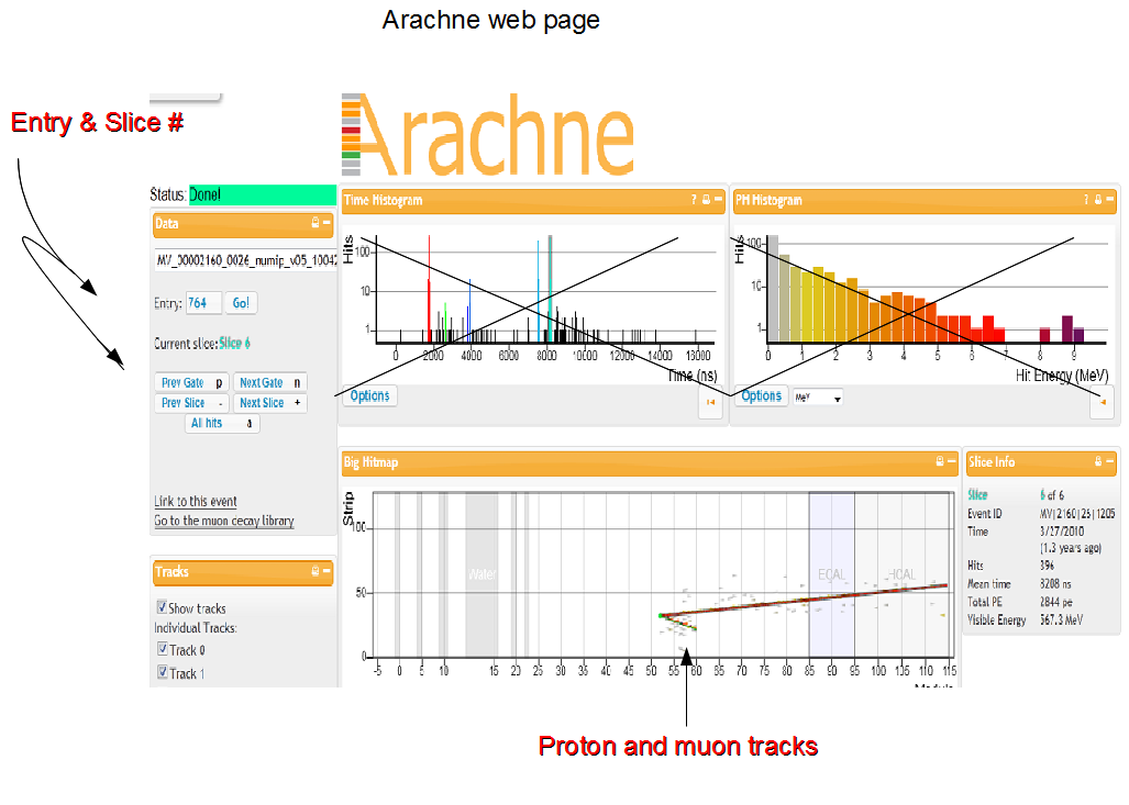
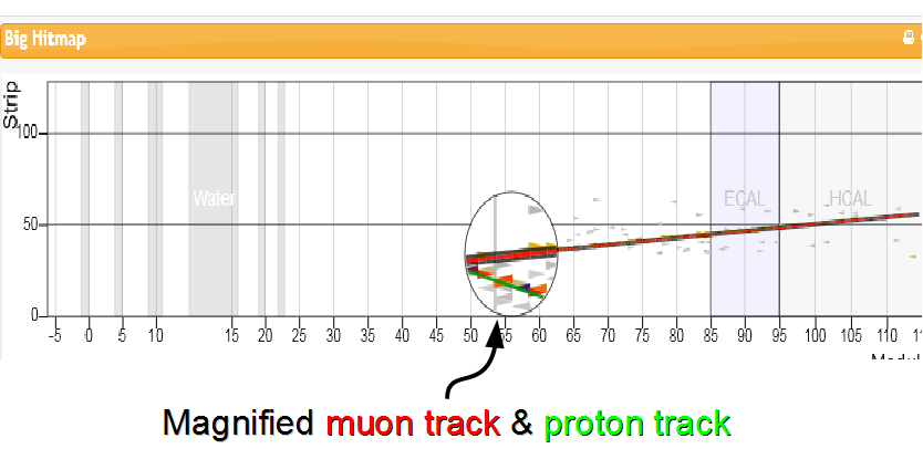
To access the Arachne program, start by clicking on the following web link.
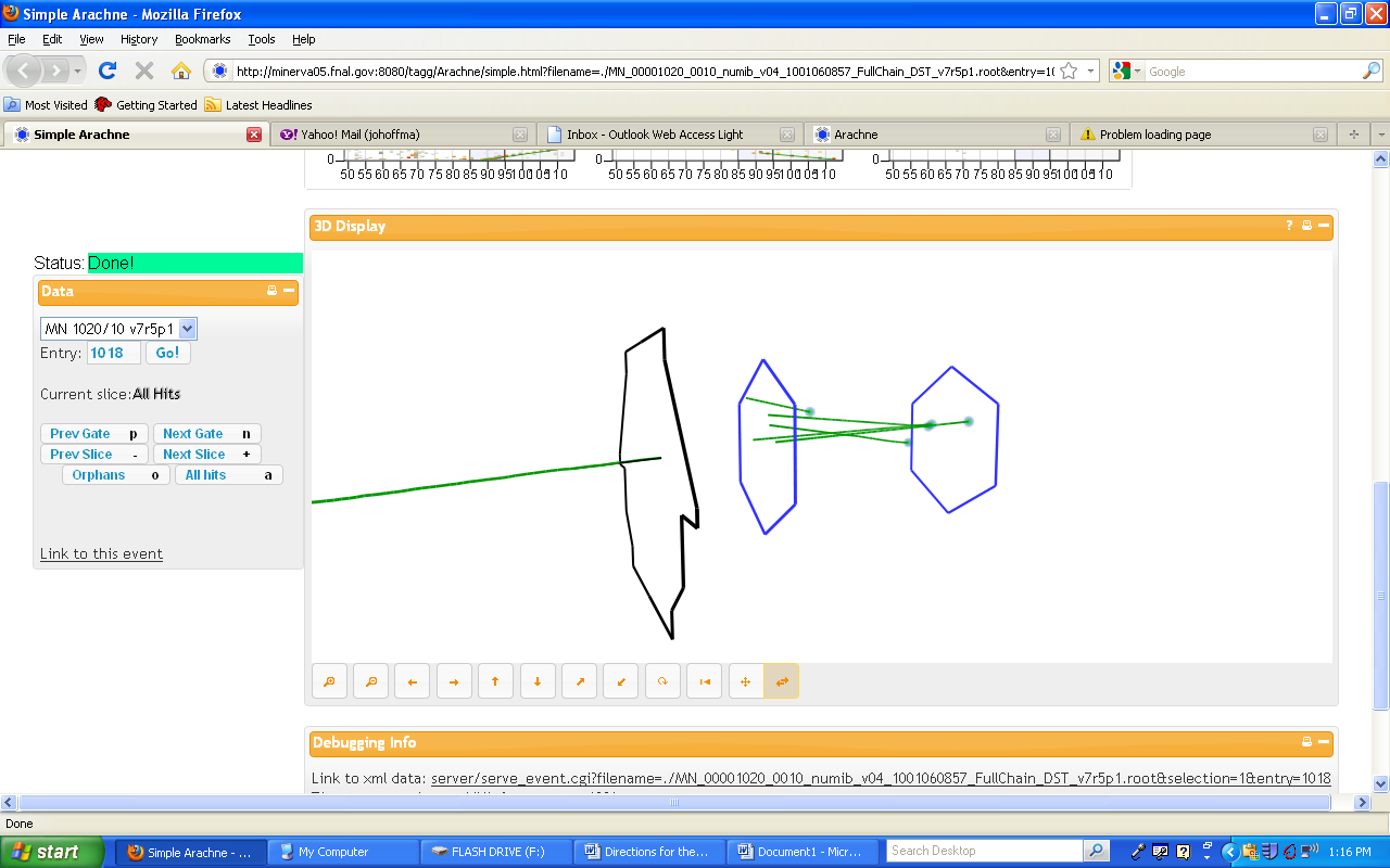
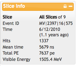
The display shows all the activity in the MINERvA detector for a single, short pulse of neutrinos. Of the few buttons on the page, you are most concerned with the “Prev slice” and “Next slice” which steps you forward and backward in time within the 16,000 nanosecond long burst of data. “All Hits” shows all the activity in this burst of particles, regardless of time.
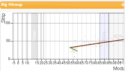
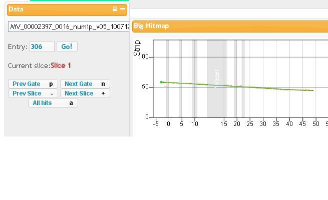
Click the ‘next slice’ button to go through each slice until you find the two special slices. First, one slice has a nice long particle that came in the front (left edge) of the detector and stopped somewhere in the middle. Second, another, later slice has a small burst of energy, maybe only a few hits, that starts right where the other long particle track ended – with no more than a one segment gap. Use magnifying glass effect to help you confirm your choice. It is also helpful to point your finger(s) at the end(s) of one or more tracks to mark its specific location, to see that it matches. Also take a look at the 3D display on the bottom (after re-clicking the all-hits button), you can see a visualization of the green reconstructed tracks that are overlaid on the activity in the detector.
Shortcut: you can type the 1-9 keys to jump to slices in the event, useful for jumping around in time.
To be concrete, after clicking Next Slice, you should see this (this is only a part of the screen, not the whole screen).
As you flip to the next slice, it looks interesting, is seems to be in almost the right spot (maybe the separation is two spaces, not one or zero). And it has only a few hits, which is right. But the visible energy is too high! It’s more than the muon’s rest energy could have given to the electron. This slice tried to fool us. Don’t worry, this rarely happens, but it is a nice lesson.
Click another two slices ahead, and here is another little burst of activity, just a few hits, located at the end of the muon track. It has a reasonable amount of energy, 34 MeV. Here is our match!
For this event you should find the long track in slice one and the small burst of energy in slice four. This is a good place to answer the first question on the worksheet.
Sometimes the slices are back to back, but more often there is a gap of several slices between the end of the first track and the continuation of the path by the electron. In muon decay, the muon travels, giving up the energy you see as the track, until it’s all gone and the muon stops. After a long while (hundreds or thousands of nanoseconds!) it decays to a Michel electron. This electron has some kinetic energy and it will continue on in some direction, it could be backwards, upwards, or any other direction. You might ask your teacher “where did the electron get its kinetic energy, if the muon had stopped and is at rest?” Teachers love questions like that, because then you all get to talk about Einstein's famous E=mc2.
The gap of several slices isn't important, but the gap in time is. Look in the box labeled “Slice Info” and notice the Mean Time (in nanoseconds) and the Visible Energy (in units of mega electron-volts MeV). Get the Mean Time for both slices, and calculate how many nanoseconds elapsed between the end of the muon and the appearance of the electron.
In the “Slice Info” box, also, get the Visible Energy for the electron from the decay. It is expected that the electron can carry between zero MeV and up to half the energy of the muon at rest, which is 107 MeV. The other energy is carried off, unseen, by two neutrinos. The final distinguishing feature of muon decay is this energy, which should be less than 60 MeV. If you think you have a splash that matches (using your finger on the screen) in space, but has more energy than this, it indicates something other than muon decay.
Look for the mean time value in the Slice information box for slice 1. That data is already entered in the appropriate data slot. We have also done that for slice 4. Note that for slice 4 you will also need the visible energy value. Subtract the mean time for the muon slice (slice 1) from the mean time for the electron slice (slice 4), in this example you get 1410 nanoseconds. Check that the data recorded on your data table matches what is shown on the Arachne screen for each slice.
The final thing you should get from the slice box is the Event ID which is MV/2397/16/575. This is a unique identification number, so you can use it to make sure you know which events you are talking about and not get them mixed up with others.
Now we can get started looking at nine more pulses of the beam at Fermilab. Go one by one through the following nine links to find the muon and its decay electron. There is one pair in each of these nine.
Muon Decay Event Two:
Muon Decay Event Three:
Muon Decay Event Four:
Muon Decay Event Five:
Muon Decay Event Six:
http://minerva05.fnal.gov/Arachne/simple.html?filename=/minerva/data/users/minervapro/outreach/muondecayDST/v10r6_2397/97/MV_00002397_0016_numip_v05_1007120650_RecoData_DST_v10r6.root&entry=668&slice=-1&phCutLow=0.5
Muon Decay Event Seven:
Muon Decay Event Eight:
Muon Decay Event Nine:
Muon Decay Event Ten::
For each one you will start with “All Hits”. Flip through the slices to find the track followed by the decay electron. Working together, determine the time (in nanoseconds) for each slice in the pair and log them in your data sheet. Make note of places where you have difficulty or questions, and work on the follow-up questions on the worksheet. Good luck, and you and your partner are on your own.
Student Chart
# | Event ID | Slice Number | Mean Time (ns) | Visible Energy (MeV) | Time Difference = #2 Mean time minus #1 Mean time | Notes and Questions |
1 | MV 2397/16/575 | 1 | 2385 ns | Example | ||
2 | 4 | 5136 ns | 34.0 MeV | 5136-2385 = 2751 ns | ||
1 | MV 2397/16/631 | 4 | ||||
2 | 6 | |||||
1 | MV 2397/16/845 | 2 | ||||
2 | 8 | |||||
1 | MV 2397/16/871 | 2 | ||||
2 | 4 | |||||
1 | MV 2397/16/921 | 4 | ||||
2 | 7 | |||||
1 | MV 2397/16/1244 | 3 | ||||
2 | 4 | |||||
1 | MV 2397/16/1453 | 2 | ||||
2 | 4 | |||||
1 | MV 2397/17/287 | 1 | ||||
2 | 7 | |||||
1 | MV 2397/17/903 | 6 | ||||
2 | 7 | |||||
1 | MV 2397/17/959 | 6 | ||||
2 | 8 |
Questions from activity Getting started finding muon decays
1. As you flip through the time-slices of Muon Decay Event One, how many have activity that is track-like? How many are small splashes of energy?
2. There were actually two time-slices in Event One, each with a small splash, which occurred at the end of the muon track. How did you know which one was the decay electron and which one to reject as some other unrelated thing?
3. Considering all eleven links, which one has the most time between the decay electron and its parent particle? Which one has the least time?
4. In addition to all the muons that stopped in the middle and decayed, what was the most interesting other thing you saw?
5. The muon you find is always traveling left to right, then stopping somewhere in the middle. How about the electrons?
6. Describe in your own words, what is radioactive decay, and specifically how does a muon decay.
This is the suggested third activity in the muon radioactive decay lessons. In this exercise, students do self-guided work to measure the muon lifetime in individual events and can observe the exponential nature of the decay.
Goals:
1. Measure a large enough sample to the exponential nature of the decay time.
2. Measure the average muon lifetime using that sample.
3. The random nature of the decay process leads to variation in mean lifetime for different samples.
Prior Knowledge:
1. Making a style of graph called a histogram of the decay time data
2. The basics of radioactive decay (from our dice activity or carbon-14 or similar.)
3. How to find decay events using the MINERvA data and Arachne.
4. Logarithms and natural logarithms often covered in Algebra-II or Pre-Calc course.
Materials:
1. Website access to Arachne and this webpage with links to many events.
2. Excel data sheet (available for download here)
3. Calculators
4. Graph paper for drawing a graph
5. Page of follow-up questions
Notes for the teacher:
Students are on their own taking data. Now that they have all practiced with the same ten events, the students (in groups probably) will be given their own set of fifteen events. There is a web page with groups of links, assign one group of links to each group of students, and make sure they know which set is theirs. Once they click on each link, they should fill out the line in the spreadsheet similar to how they did in the previous activity, including the event ID, the muon and electron time, and the electron energy. There is other information available to record, but it isn't necessary.
Filling out and combining the spreadsheets: Not only will the students calculate a decay time from their fifteen events, but this activity works best if you have a means of combining all their spreadsheet information into one large spreadsheet, and thus creating a very large data set. This means that you should consider your computer lab setup. If there are enough computers for teams to sit side by side at two different computers, entering data in the spreadsheet at the same time as they view it on the next computer works well. You can also have students jot down data on a hard copy and then flip between applications to enter it as they go as well. Otherwise, determine where in the process you would like them to enter data in the spreadsheet and be sure that students are clear on where they should do that.
After students have collected their data, they will be instructed to analyze their small set of data for average lifetime and half-life. You should expect quite a bit of variation in the data obtained from this small data set. They will compare their answers with three other groups to see what kind of variation there is in the data sets. You can choose to stop students and do some analysis at this point in the process, and talk about the difficulties with small data sets and variations in results. You may want to wait until all have completed their data analysis of both their small group and whole class set, this will depend on the type of student groups you are working with, and whether they will need some additional reinforcement that they are on the right track before proceeding to the next part of the activity.
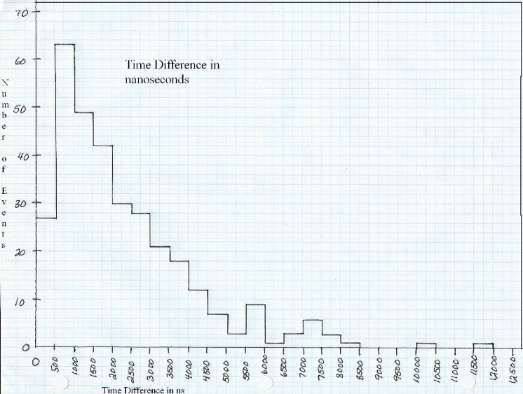
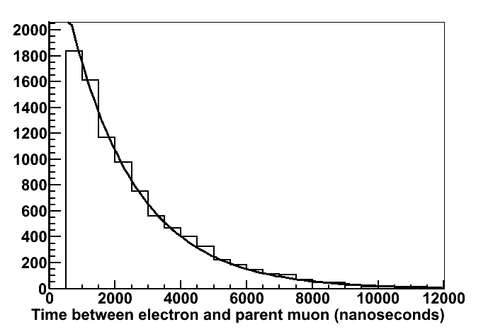
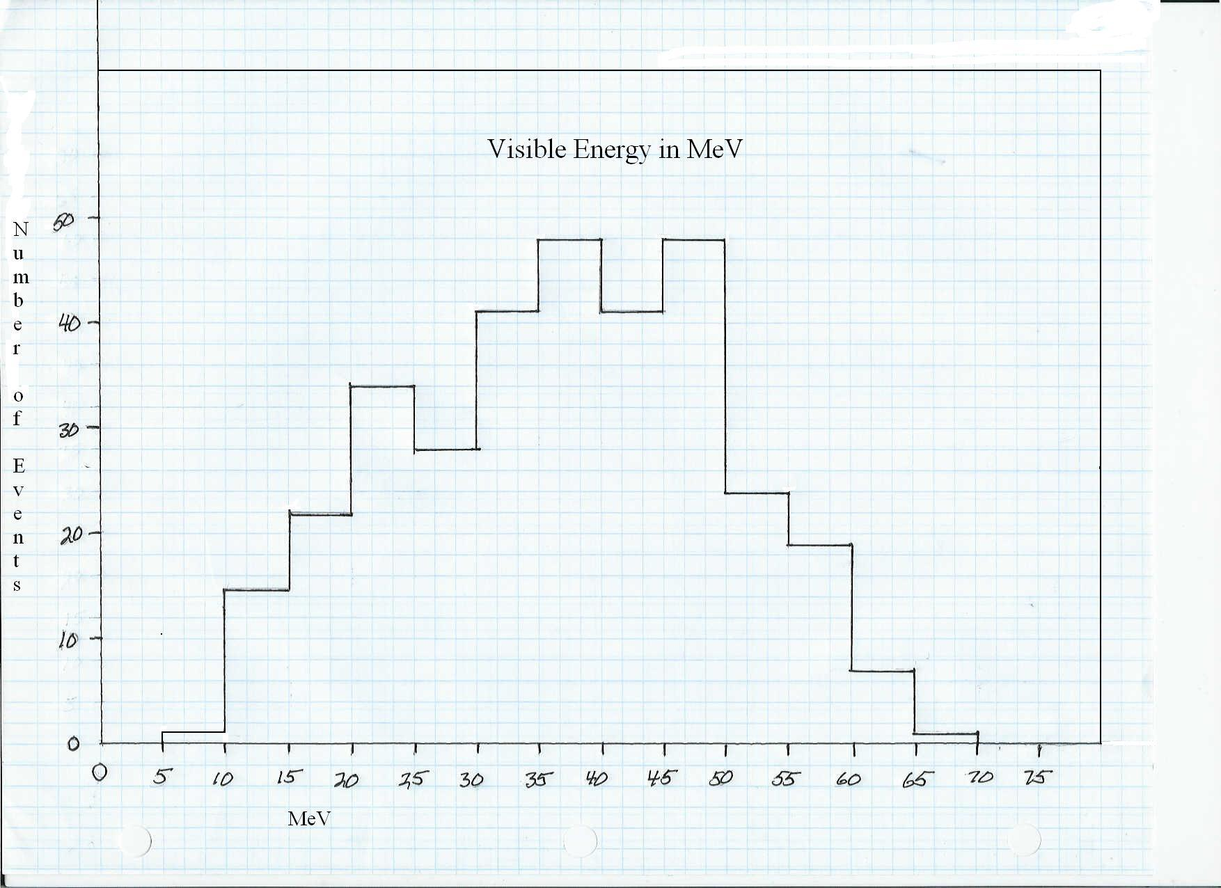
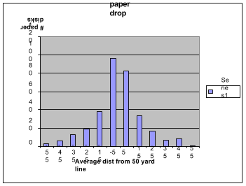
Histograms: Students will be making a couple of histogram style graphs. You might want to allow them to determine their own parameters for graphing, or for ease of class discussion choose to have them use the same scale. Intervals of 500 nanoseconds in decay time works fairly well. The graph below shows a sample of data.
Measurement uncertainty: The results that students get for average lifetimes and half-lives are likely to vary fairly dramatically. This is of course due to small sample size. The same issue is also present in familiar contexts like political polling, for example. Comparing the whole group sample size to the small individual groupings is a good discussion, and is part of the activity.
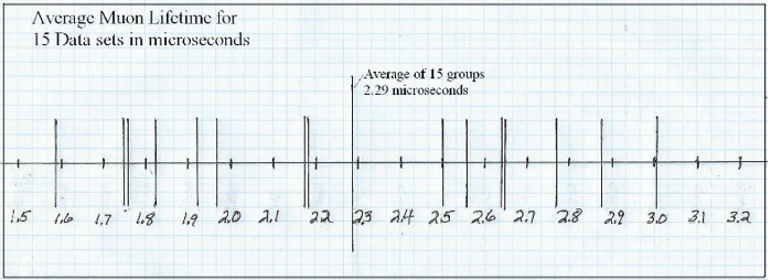
A step further is to take a look at the average lifetime data calculated by the individual groups, and calculate how much the data vary. This will be reassuring to those students who are likely to think that a value different from the “so called” right answer is wrong. The uncertainty of decay is an important concept in the bigger scientific picture that clearly tells us that things don't always fall exactly as a single accepted value says they should have. An easy way to do this in the classroom is to set up a range line on the board (see example graph below) and have students place their groups calculated value for average lifetime on the scale and include the value. Then it is an easy job to take the average of all of the individual group results, find the range of measurement variance, the largest variance from the average value is your error range. This is a reasonable estimate of event variance. If you would like to take your class further in this discussion you can Google ‘standard deviation calculation’. You may have a student ideally suited for a little extra job along these lines.
Computing mean life, simple and not simple: It is reasonable, and mostly correct, to simply calculate the mean life by making the average of the data and be done. There is actually a subtle problem with this activity, and you can decide whether you want your class to realize the problem and correct for it, or enjoy the new concepts they learned without worrying about the subtle thing. You or your students may (will?) notice that there are no decays with decay time less than 500 nanoseconds. There is a technical issue with how MINERvA records data that causes it to record data very short times after the muon in a different way (that we can't measure with Arachne), or even not record it at all. Because of this, we have hidden any decays that happen sooner than 500 nanoseconds. But wait! For an exponential decay, that’s the interval that has the most decays! If they are not there, isn't that going to make our mean life too high?
Well, it won’t be so very high that the students will notice or think they are getting the “wrong” answer. So no harm is done? Or you can consider two ways of correcting it. The boring but effective way, but one that is often used by practicing scientists, is to estimate what events were missing from that first interval, include that estimate into your average, and consider that the more accurate number with some uncertainty because your estimate probably wasn’t perfect. Okay, this is totally valid, as long as you include that in your discussion of the results.
The interesting argument that leads to a correction to the average lifetime invokes an understanding of the dice activity in a very special way. If you want your students to try it, cut and paste the following thing into the instructions and questions for your students.
[For students: if the teacher wants them to consider it.]
There is a problem here, there is data missing between 0 and 500 ns. That’s actually the interval where we expect most of the events to be, so our average will be too high by a little bit. But the fix is interesting. Remember the dice activity, especially the version where you threw 100 dice at the same time, and separated out those with a “one”, and then rolled again? Each time you rolled, it was the same random 1/6 chance, the dice don’t remember how many rolls went by without decaying. You could have ignored that first roll, and just as well pretended you had started out with roughly 85 dice. Or maybe you didn’t know it, but there was a prior roll you didn’t see that had 115 dice, and you walked in with only 100 left. Your analysis of the lifetime for the dice wouldn’t have been affected by it.
Likewise, we can analyze the average lifetime of the muons as if those that decayed in the first interval never happened, and the lifetime clock started 500 nanoseconds later, for the second roll. If this is convincing, then mathematically we have two (equivalent) choices. Either subtract 500 nanoseconds from every event we are putting into the mean lifetime calculation, or subtract 500 nanoseconds from the average. Do you see that these two are equivalent? If you do, then the latter choice is easier, and will give you a more accurate measurement.
Looking at only student small group results should result in an average lifetime for muons of 2.29 μs. Note this is converted from the nanoseconds used in the graphing activity to microseconds- just move the decimal three places to the left. The average muon half-life should be somewhere in the range of 1.56 μs.
If all of the student groups’ average time difference is calculated we get a range of times from 1.591 to 3.079 μs. The largest difference is 0.793 μs providing the error range for this set of data. The next step asks students to make the same calculations using the whole group data. The data yields 2.32 μs for the average lifetime in this scenario, and an half-life of 1.61 μs. Graphs below for time difference, show the distribution for the assigned group data at the time of writing this guide.
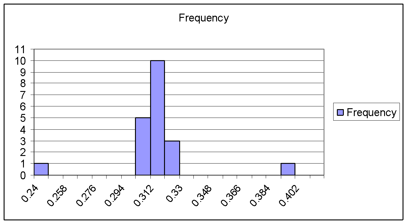
This trend with increased data, the exponential shape becomes more clear, and the mean lifetime measurement is more accurate, can be taken to its logical extreme, if only you have the time or some way to automate the process (or both). Here is the equivalent histogram for a very large data set, about 10,000 events, which include exactly the same decay events you measured, but also include four months of data in spring and summer 2010. You can use this histogram you’re your students if you want them to better see how lots of data overcomes the random fluctuations inherent in the smaller samples.
Teacher Answer Key – Note: the first 10 events are from the previous activity The visible energy and times listed in this table might differ a little bit from the one in Arachne because of software and calibration updates that happened after this answer key was made. The results of you and your student’s studies will still work.
Event ID | Entry Number | Slice Numbers | MTime 1 (ns) | Mtime 2 (ns) | Vis. Energy (MeV) | Time difference | Notes/Questions |
MV 2397/16/575 | 1-4 | 2385 | 5136 | 34 | 2751 |
| |
MV 2397/16/637 |
| 4-6 | 6069 | 7340 | 40.1 | 1271 |
|
MV 2397/16/845 |
| 2-8 | 4010 | 9339 | 24.3 | 5329 |
|
MV 2397/16/871 |
| 2-4 | 8823 | 10489 | 20.3 | 1666 |
|
MV 2397/16/921 |
| 4-7 | 4287 | 11164 | 30.4 | 6877 |
|
MV 2397/16/1244 |
| 3-4 | 4357 | 5840 | 25.3 | 1483 |
|
MV 2397/16/1453 |
| 2-4 | 4042 | 5117 | 58.9 | 1075 |
|
MV 2397/17/287 |
| 1-7 | 2462 | 6068 | 29 | 3606 |
|
MV 2397/17/903 |
| 6-7 | 7641 | 8770 | 15 | 1129 |
|
MV 2397/17/959 |
| 8-9 | 7979 | 10362 | 37.4 | 2383 |
|
|
|
|
|
|
|
|
|
MV 2063/1/770 |
| 2-3 | 4138 | 4959 | 26.6 | 821 |
|
MV 2063/2/574 |
| 2-3 | 2659 | 3325 | 47.4 | 666 |
|
MV 2063/2/798 |
| 2-5 | 6226 | 8580 | 48.1 | 2354 |
|
MV 2063/2/856 |
| 14-15 | 9712 | 14093 | 31.6 | 4381 |
|
MV 2063/2/980 |
| 6-9 | 7345 | 11789 | 12.6 | 4444 |
|
MV 2063/3/970 |
| 4-6 | 8338 | 10084 | 17.4 | 1746 |
|
MV 2063/4/146 |
| 4-7 | 4213 | 6808 | 37.2 | 2595 |
|
MV 2063/4/840 |
| 3-4 | 2978 | 3736 | 38.8 | 758 |
|
MV 2063/4/980 |
| 2-3 | 2120 | 3095 | 31.7 | 975 |
|
MV 2063/5/346 |
| 2-8 | 3283 | 7462 | 25.9 | 4179 |
|
MV 2063/5/954 |
| 2-6 | 2772 | 6857 | 46.5 | 4085 |
|
MV 2063/6/128 |
| 8-9 | 7040 | 8250 | 35.7 | 1210 |
|
MV 2063/6/558 |
| 9-13 | 7546 | 10157 | 43.3 | 2611 |
|
MV 2063/7/322 |
| 1-2 | 2264 | 3314 | 46.2 | 1050 |
|
MV 2063/8/500 |
| 5-10 | 6740 | 9525 | 34.6 | 2785 |
|
|
|
|
|
|
|
|
|
MV 2063/8/534 |
| 1-4 | 5616 | 7351 | 42.7 | 1735 |
|
MV 2063/8/586 |
| 7-15 | 4768 | 8668 | 28.9 | 3900 |
|
MV 2063/8/696 |
| 5-7 | 5416 | 10574 | 42.6 | 5158 |
|
MV 2063/8/760 |
| 10-15 | 6183 | 12122 | 34.8 | 5939 |
|
MV 2063/8/888 |
| 3-4 | 2801 | 3361 | 37.3 | 560 |
|
MV 2063/9/296 |
| 8-9 | 8694 | 11323 | 42.5 | 2629 |
|
MV 2063/9/308 |
| 5-12 | 5486 | 12229 | 34.6 | 6743 |
|
MV 2063/9/318 |
| 12-13 | 9612 | 12880 | 36.1 | 3268 |
|
MV 2063/9/626 |
| 13-14 | 8337 | 9333 | 25 | 996 |
|
MV 2063/10/26 |
| 4-8 | 4872 | 11188 | 27.3 | 6316 |
|
MV 2063/10/118 |
| 7-13 | 5086 | 7973 | 15.4 | 2887 |
|
MV 2063/10/818 |
| 5-8 | 6656 | 7758 | 27.3 | 1102 |
|
MV 2063/11/180 |
| 5-7 | 6047 | 6788 | 35.3 | 741 |
|
MV 2063/11/192 |
| 5-7 | 5458 | 8337 | 32.5 | 2879 |
|
MV 2063/11/906 |
| 8-10 | 6037 | 7119 | 35.8 | 1082 |
|
|
|
|
|
|
|
|
|
MV 2063/12/312 |
| 7-9 | 8487 | 13195 | 45 | 4708 |
|
MV 2063/12/834 |
| 5-13 | 3704 | 13284 | 41.2 | 9580 |
|
MV 2064/1/24 |
| 2-7 | 3738 | 6299 | 47.7 | 2561 |
|
MV 2064/1/34 |
| 7-10 | 5539 | 7005 | 35.9 | 1466 |
|
MV 2064/1/414 |
| 1-4 | 3751 | 6940 | 27.7 | 3189 |
|
MV 2064/1/782 |
| 2-3 | 2498 | 3058 | 47.6 | 560 |
|
MV 2064/1/1042 |
| 2-3 | 3998 | 4496 | 29.1 | 498 |
|
MV 2064/1/1042 |
| 4-12 | 5130 | 8881 | 18 | 3751 |
|
MV 2064/1/1056 |
| 7-13 | 5962 | 11946 | 19.6 | 5984 |
|
MV 2064/3/588 |
| 6-8 | 5660 | 6143 | 14.2 | 483 |
|
MV 2064/3/598 |
| 4-6 | 2254 | 3115 | 33.3 | 861 |
|
MV 2064/3/1046 |
| 7-10 | 7064 | 10145 | 50.6 | 3081 |
|
MV 2064/4/736 |
| 4-9 | 5097 | 9765 | 33.8 | 4668 |
|
MV 2064/5/190 |
| 6-9 | 7572 | 10583 | 37.3 | 3011 |
|
MV 2064/5/226 |
| 1-3 | 2252 | 3646 | 43.6 | 1394 |
|
MV 2064/5/380 |
| 2-6 | 5739 | 8635 | 32 | 2896 |
|
|
|
|
|
|
|
|
|
MV 2064/5/532 |
| 2-5 | 2762 | 3463 | 38.9 | 701 |
|
MV 2064/5/918 |
| 1-3 | 2146 | 3704 | 37.6 | 1558 |
|
MV 2064/5/1034 |
| 4-7 | 6752 | 8654 | 16.3 | 1902 |
|
MV 2064/6/570 |
| 1-2 | 1923 | 2554 | 40.8 | 631 |
|
MV 2064/6/750 |
| 8-11 | 7587 | 10214 | 34.4 | 2627 |
|
MV 2065/2/128 |
| 3-7 | 5557 | 8256 | 46.9 | 2699 |
|
MV 2065/2/186 |
| 6-7 | 9258 | 9827 | 44 | 569 |
|
MV 2065/2/526 |
| 2-8 | 6924 | 11125 | 31.2 | 4201 |
|
MV 2065/2/544 |
| 2-6 | 3235 | 5947 | 45.7 | 2712 |
|
MV 2065/3/422 |
| 2-5 | 2573 | 3722 | 46.4 | 1149 |
|
MV 2065/3/594 |
| 12-13 | 9162 | 10388 | 42.5 | 1226 |
|
MV 2065/3/904 |
| 3-7 | 2906 | 6765 | 24.4 | 3859 |
|
MV 2065/3/998 |
| 8-13 | 7266 | 11733 | 44.1 | 4467 |
|
MV 2067/1/116 |
| 1-6 | 2164 | 4396 | 22.7 | 2232 |
|
MV 2067/1/320 |
| 7-11 | 6288 | 12499 | 28.7 | 6211 |
|
|
|
|
|
|
|
|
|
MV 2067/1/1010 |
| 6-7 | 7635 | 12222 | 45.7 | 4587 |
|
MV 2067/2/154 |
| 1-4 | 2738 | 4259 | 33.1 | 1521 |
|
MV 2067/2/706 |
| 6-11 | 5513 | 12303 | 40.1 | 6790 |
|
MV 2067/3/84 |
| 1-7 | 2045 | 13224 | 28.9 | 11179 |
|
MV 2067/3/276 |
| 11-15 | 7741 | 9896 | 12.2 | 2155 |
|
MV 2067/4/740 |
| 4-8 | 5083 | 8097 | 25.5 | 3014 |
|
MV 2067/4/1014 |
| 4-7 | 5870 | 7501 | 26.3 | 1631 |
|
MV 2067/4/1108 |
| 3-4 | 5983 | 6501 | 45.3 | 518 |
|
MV 2067/4/1164 |
| 1-6 | 3013 | 6925 | 47.2 | 3912 |
|
MV 2067/5/108 |
| 10-11 | 9353 | 12744 | 13.7 | 3391 |
|
MV 2067/5/748 |
| 8-9 | 7473 | 9496 | 36.1 | 2023 |
|
MV 2067/6/226 |
| 3-4 | 7995 | 8498 | 36.7 | 503 |
|
MV 2067/6/606 |
| 2-5 | 2336 | 3498 | 40.3 | 1162 |
|
MV 2067/6/690 |
| 1-2 | 2355 | 2907 | 28.4 | 552 |
|
MV 2067/6/832 |
| 3-6 | 7258 | 14557 | 31 | 7299 |
|
|
|
|
|
|
|
|
|
MV 2067/6/1060 |
| 11-13 | 8524 | 11992 | 45.4 | 3468 |
|
MV 2067/7/216 |
| 1-2 | 1861 | 2394 | 27.9 | 533 |
|
MV 2067/8/788 |
| 6-8 | 7243 | 10829 | 41.4 | 3586 |
|
MV 2067/68/802 |
| 6-7 | 7393 | 13841 | 35 | 6448 |
|
MV 2067/8/924 |
| 2-10 | 3567 | 7707 | 21.9 | 4140 |
|
MV 2067/8/976 |
| 7-8 | 7693 | 10347 | 16.9 | 2654 |
|
MV 2067/9/86 |
| 10-11 | 7116 | 7955 | 30.2 | 839 |
|
MV 2067/9/174 |
| 9-11 | 8330 | 9711 | 26.2 | 1381 |
|
MV 2067/89/220 |
| 8-11 | 5663 | 7431 | 22.1 | 1768 |
|
MV 2067/9/718 |
| 8-10 | 7503 | 11474 | 15.8 | 3971 |
|
MV 20679/760 |
| 4-5 | 5201 | 6722 | 27.5 | 1521 |
|
MV 2067/10/146 |
| 12-14 | 7468 | 13814 | 48.4 | 6346 |
|
MV 2067/10/1048 |
| 5-8 | 4142 | 7390 | 39.5 | 673 |
|
MV 2067/10/1152 |
| 5-7 | 4712 | 7939 | 26.7 | 3227 |
|
MV 2067/11//90 |
| 9-12 | 7887 | 10961 | 39.7 | 3074 |
|
|
|
|
|
|
|
|
|
MV 2067/11/872 |
| 6-8 | 5491 | 6115 | 21.7 | 624 |
|
MV 2067/11/896 |
| 4-6 | 5491 | 8458 | 32.4 | 2967 |
|
MV 2067/11/896 |
| 2-8 | 3447 | 9891 | 7.6 | 6444 |
|
MV 2067/12/92 |
| 1-5 | 2158 | 4757 | 40.6 | 2599 |
|
MV 2067/12/92 |
| 2-4 | 2768 | 4174 | 17.4 | 1406 |
|
MV 2067/12/322 |
| 6-7 | 8977 | 9815 | 35.6 | 838 |
|
MV 2067/13/2 |
| 4-5 | 4491 | 5138 | 35.1 | 647 |
|
MV 2067/13/268 |
| 4-8 | 5613 | 15026 | 20.1 | 9413 |
|
MV 2067/13/448 |
| 5-10 | 6663 | 10384 | 19.2 | 3721 |
|
MV 2067/13/490 |
| 3-8 | 4384 | 7466 | 35.6 | 3082 |
|
MV 2067/13/514 |
| 6-12 | 5819 | 8295 | 29 | 2476 |
|
MV 2067/13/826 |
| 6-7 | 6286 | 6787 | 43.2 | 501 |
|
MV 2067/14/274 |
| 1-2 | 2526 | 3652 | 25 | 1126 |
|
MV 2067/14/448 |
| 6-8 | 5928 | 8161 | 40 | 2233 |
|
MV 2067/14/522 |
| 4-5 | 4260 | 4788 | 36.2 | 528 |
|
MV 2067/14/1074 |
| 3-7 | 3035 | 5107 | 35.6 | 2072 |
|
MV 2067/15/188 |
| 2-5 | 5371 | 8130 | 34.9 | 2759 |
|
|
|
|
|
|
|
|
|
MV 2067/15/694 |
| 11-12 | 8768 | 10287 | 41.3 | 1519 |
|
MV 2067/15/842 |
| 4-7 | 4879 | 6243 | 21.6 | 1364 |
|
MV 2067/15/1014 |
| 4-9 | 5702 | 10800 | 11.6 | 5098 |
|
MV 2067/15/1034 |
| 3-4 | 2731 | 3910 | 26.7 | 1179 |
|
MV 2067/16/394 |
| 6-8 | 7578 | 8392 | 18.5 | 814 |
|
MV 2067/16/488 |
| 1-4 | 2963 | 4445 | 30.2 | 1482 |
|
MV 2067/16/518 |
| 5-7 | 5661 | 7076 | 55.4 | 1415 |
|
MV 2067/17/272 |
| 5-7 | 6280 | 12780 | 32.3 | 6500 |
|
MV 2067/17/606 |
| 2-7 | 2458 | 8136 | 35.4 | 5678 |
|
MV 2071/1/6 |
| 5-9 | 7035 | 10443 | 44.9 | 3408 |
|
MV 2071/1/1004 |
| 2-4 | 2332 | 4095 | 16.6 | 1763 |
|
MV 2071/2/58 |
| 8-9 | 9502 | 10134 | 32.8 | 632 |
|
MV 2071/2/498 |
| 3-5 | 6057 | 6615 | 24.2 | 558 |
|
MV 2071/3/162 |
| 7-8 | 7331 | 8965 | 32 | 1634 |
|
MV 2071/3/258 |
| 4-6 | 4042 | 4637 | 12.4 | 595 |
|
MV 2071/3/258 |
| 5-7 | 4477 | 5548 | 21.3 | 1071 |
|
|
|
|
|
|
|
|
|
MV 2071/3/818 |
| 2-3 | 3106 | 3975 | 43.5 | 869 |
|
MV 2071/3/1064 |
| 8-11 | 6826 | 9231 | 17.7 | 2405 |
|
MV 2071/4/64 |
| 3-9 | 2549 | 6577 | 25.2 | 4028 |
|
MV 2071/4/404 |
| 1-2 | 1882 | 2658 | 14.1 | 776 |
|
MV 2071/4/404 |
| 9-10 | 9259 | 9963 | 10.1 | 704 |
|
MV 2071/4/640 |
| 1-5 | 3185 | 5624 | 56.8 | 2439 |
|
MV 2071/4/726 |
| 4-5 | 8001 | 9526 | 43.8 | 1525 |
|
MV 2071/5/54/ |
| 3-6 | 6384 | 9031 | 29.6 | 2647 |
|
MV 2071/5/1104 |
| 3-5 | 6401 | 7029 | 46.8 | 628 |
|
MV 2071/6/372 |
| 6-8 | 5372 | 6780 | 29.6 | 1408 |
|
MV 2071/6/476 |
| 6-7 | 6213 | 7368 | 47.7 | 1155 |
|
MV 2071/6/498 |
| 3-4 | 2660 | 4756 | 32.3 | 2096 |
|
MV 2071/6/818 |
| 2-5 | 3425 | 6038 | 14.8 | 2613 |
|
MV 2071/6/1032 |
| 7-9 | 6928 | 7771 | 30.9 | 843 |
|
MV 2071/6/1148 |
| 6-10 | 6354 | 8526 | 41.4 | 2172 |
|
MV 2071/7/32 |
| 6-7 | 4836 | 6738 | 44 | 1902 |
|
|
|
|
|
|
|
|
|
MV 2071/7/580 |
| 3-4 | 2877 | 3521 | 46.7 | 644 |
|
MV 2071/7/652 |
| 4-6 | 3709 | 8489 | 26.7 | 4780 |
|
MV 2071/7/1166 |
| 8-9 | 5351 | 8102 | 48.4 | 2751 |
|
MV 2071/8/894 |
| 5-7 | 5843 | 6705 | 44.9 | 862 |
|
MV 2071/8/912 |
| 6-8 | 5828 | 7406 | 28.3 | 1578 |
|
MV 2071/8/1194 |
| 6-9 | 8075 | 15103 | 48.5 | 7028 |
|
MV 2071/9/350 |
| 4-6 | 7292 | 8240 | 33.4 | 948 |
|
MV 2071/9/978 |
| 7-12 | 5978 | 12599 | 24.1 | 6621 |
|
MV 2071/9/1136 |
| 7-9 | 6929 | 7774 | 42.2 | 845 |
|
MV 2071/10/28 |
| 15-16 | 9746 | 13636 | 29.4 | 3890 |
|
MV 2071/10/412 |
| 1-2 | 3271 | 3842 | 22.3 | 571 |
|
MV 2071/11/44 |
| 8-10 | 6356 | 7567 | 16.5 | 1211 |
|
MV 2071/11/44 |
| 12-13 | 9233 | 10540 | 43.6 | 1307 |
|
MV 2071/11/810 |
| 1-4 | 2445 | 6845 | 46.4 | 4400 |
|
MV 2071/12/156 |
| 2-3 | 2011 | 2511 | 33.4 | 500 |
|
MV 2071/12/226 |
| 3-4 | 7667 | 9232 | 40 | 1565 |
|
|
|
|
|
|
|
|
|
MV 2071/12/268 |
| 11-12 | 7081 | 8705 | 19 | 1624 |
|
MV 2071/12/752 |
| 3-4 | 6625 | 8512 | 27.4 | 1887 |
|
MV 2071/13/310 |
| 2-4 | 2460 | 3647 | 38.9 | 1187 |
|
MV 2071/13/948 |
| 3-9 | 3084 | 7210 | 29.5 | 4126 |
|
MV 2071/14/204 |
| 6-8 | 9028 | 11535 | 27.9 | 2507 |
|
MV 2071/14/340 |
| 1-13 | 1935 | 11411 | 28.1 | 9476 |
|
MV 2071/14/942 |
| 4-8 | 4194 | 7416 | 57.3 | 3222 |
|
MV 2071/14/1142 |
| 2-6 | 2180 | 3148 | 30 | 968 |
|
MV 2071/15/766 |
| 2-5 | 4230 | 6337 | 19.7 | 2107 |
|
MV 2071/15/808 |
| 9-10 | 7980 | 10793 | 13.2 | 2813 |
|
MV 2071/15/852 |
| 8-12 | 6143 | 9590 | 44.2 | 3447 |
|
MV 2071/15/884 |
| 1-2 | 1835 | 2781 | 21.9 | 946 |
|
MV 2071/15/1034 |
| 1-4 | 2304 | 5877 | 25.4 | 3573 |
|
MV 2071/16/172 |
| 7-8 | 8106 | 13192 | 24.4 | 5086 |
|
MV 2071/16/258 |
| 11-13 | 8605 | 12523 | 36 | 3918 |
|
|
|
|
|
|
|
|
|
MV 2071/16/388 |
| 5-9 | 4851 | 8598 | 42.5 | 3747 |
|
MV 2071/16/440 |
| 8-12 | 6929 | 12141 | 22.6 | 5212 |
|
MV 2071/16/1028 |
| 7-8 | 6326 | 9680 | 51.2 | 3354 |
|
MV 2071/16/1036 |
| 9-13 | 7922 | 11034 | 16.8 | 3112 |
|
MV 2071/17/746 |
| 9-11 | 6698 | 8519 | 41.3 | 1821 |
|
MV 2071/17/950 |
| 1-5 | 2283 | 5129 | 53.5 | 2846 |
|
MV 2071/18/16 |
| 3-8 | 4689 | 10679 | 36.6 | 5990 |
|
MV 2071/18/412 |
| 4-6 | 7729 | 9142 | 25 | 1413 |
|
MV 2071/18/952 |
| 4-9 | 2970 | 5759 | 50 | 2789 |
|
MV 2071/20/304 |
| 6-8 | 7279 | 8710 | 15 | 1431 |
|
MV 2071/20/402 |
| 3-6 | 5561 | 8284 | 42.7 | 2723 |
|
MV 2071/20/458 |
| 4-7 | 6726 | 8456 | 15.7 | 1730 |
|
MV 2071/20/702 |
| 5-15 | 5667 | 10791 | 35.4 | 5124 |
|
MV 2071/20/764 |
| 8-9 | 9536 | 12920 | 22.6 | 3384 |
|
MV 2071/21/208 |
| 1-2 | 1818 | 2486 | 22.3 | 668 |
|
MV 2071/21/208 |
| 11-14 | 7939 | 8749 | 22.8 | 810 |
|
|
|
|
|
|
|
|
|
MV 2071/21/634 |
| 6-7 | 7795 | 10120 | 24.4 | 2325 |
|
MV 2071/22/116 |
| 9-10 | 6100 | 8030 | 21.6 | 1930 |
|
MV 2071/22/116 |
| 13-14 | 9180 | 12341 | 26.8 | 3161 |
|
MV 2071/22/494 |
| 4-5 | 3084 | 3826 | 38.2 | 742 |
|
MV 2071/22/804 |
| 7-9 | 9014 | 11316 | 32.9 | 2302 |
|
MV 2071/23/618 |
| 4-6 | 4800 | 5656 | 41 | 856 |
|
MV 2071/23/586 |
| 4-6 | 6943 | 8915 | 38.8 | 1972 |
|
MV 2071/24/714 |
| 11-16 | 6685 | 9467 | 29.5 | 2782 |
|
MV 2071/25/276 |
| 10-12 | 7934 | 10310 | 47.7 | 2376 |
|
MV 2071/25/680 |
| 5-7 | 4515 | 5970 | 26.5 | 1455 |
|
MV 2071/26/382 |
| 1-5 | 1898 | 4728 | 29.7 | 2830 |
|
MV 2071/26/886 |
| 5-12 | 5620 | 11612 | 33.3 | 5992 |
|
MV 2072/2/878 |
| 5-7 | 7745 | 10972 | 38.8 | 3227 |
|
MV 2072/2/1042 |
| 3-5 | 4033 | 5208 | 23.2 | 1175 |
|
MV 2072/2/1178 |
| 7-14 | 6221 | 9226 | 30 | 3005 |
|
MV 2072/3/118 |
| 2-4 | 2636 | 3896 | 56.6 | 1260 |
|
|
|
|
|
|
|
|
|
MV 2072/3/238 |
| 7-8 | 8772 | 9817 | 30.8 | 1045 |
|
MV 2072/3/306 |
| 6-8 | 7359 | 9457 | 33 | 2098 |
|
MV 2072/3/426 |
| 2-5 | 2954 | 5402 | 27.7 | 1137 |
|
MV 2072/3/580 |
| 5-6 | 4472 | 5261 | 27.7 | 789 |
|
MV 2072/3/922 |
| 4-5 | 8359 | 14838 | 25.5 | 6479 |
|
MV 2072/4/582 |
| 5-11 | 5312 | 8468 | 33 | 3156 |
|
MV 2072/4/582 |
| 12-13 | 9047 | 11409 | 33.3 | 2362 |
|
MV 2072/4/624 |
| 5-6 | 5201 | 5770 | 22.2 | 569 |
|
MV 2072/5/336 |
| 15-18 | 7874 | 11111 | 26.2 | 3237 |
|
MV 2072/5/734 |
| 16-19 | 7985 | 10442 | 35.6 | 2457 |
|
MV 2072/5/1056 |
| 8-10 | 6954 | 8305 | 26.4 | 1351 |
|
MV 2072/6/108 |
| 10-11 | 9426 | 10979 | 32.6 | 1553 |
|
MV 2072/6/330 |
| 7-8 | 6955 | 13229 | 41.1 | 6274 |
|
MV 2072/7/834 |
| 9-11 | 7540 | 13188 | 25.7 | 5648 |
|
MV 2072/8/114 |
| 9-11 | 7582 | 13106 | 43.7 | 5524 |
|
MV 2072/8/608 |
| 9-10 | 8439 | 9099 | 49.4 | 660 |
|
|
|
|
|
|
|
|
|
MV 2072/8/848 |
| 2-4 | 3194 | 6955 | 35.4 | 3761 |
|
MV 2072/8/944 |
| 3-5 | 6857 | 13040 | 18.1 | 6183 |
|
MV 2072/8/944 |
| 1-6 | 4299 | 14064 | 29.8 | 9765 |
|
MV 2072/9/712 |
| 2-3 | 2662 | 3756 | 25.8 | 1094 |
|
MV 2072/9/1014 |
| 3-5 | 4367 | 5220 | 34.1 | 853 |
|
MV 2072/9/1180 |
| 3-4 | 2704 | 3453 | 49.1 | 749 |
|
MV 2072/10/212 |
| 8-12 | 7234 | 9429 | 28.8 | 2195 |
|
MV 2072/10/212 |
| 10-13 | 7890 | 9605 | 24.1 | 1715 |
|
MV 2072/10/572 |
| 3-4 | 5345 | 6916 | 39.5 | 1571 |
|
MV 2072/10/698 |
| 9-10 | 9704 | 11371 | 13.1 | 1667 |
|
MV 2072/11/352 |
| 6-7 | 6008 | 8390 | 14.4 | 2382 |
|
MV 2072/11/416 |
| 6-8 | 7627 | 10454 | 40.9 | 2827 |
|
MV 2072/11/818 |
| 6-9 | 7623 | 11639 | 28.2 | 4016 |
|
MV 2072/11/1020 |
| 2-7 | 2909 | 7206 | 34.7 | 4297 |
|
MV 2072/11/1096 |
| 8-12 | 6676 | 11789 | 29.8 | 5113 |
|
MV 2072/12/224 |
| 2-6 | 3075 | 5098 | 13.4 | 2023 |
|
MV 2072/13/678 |
| 4-12 | 4575 | 11090 | 50.7 | 6515 |
|
Instructions for students:
General Instructions- Work with a partner for this activity
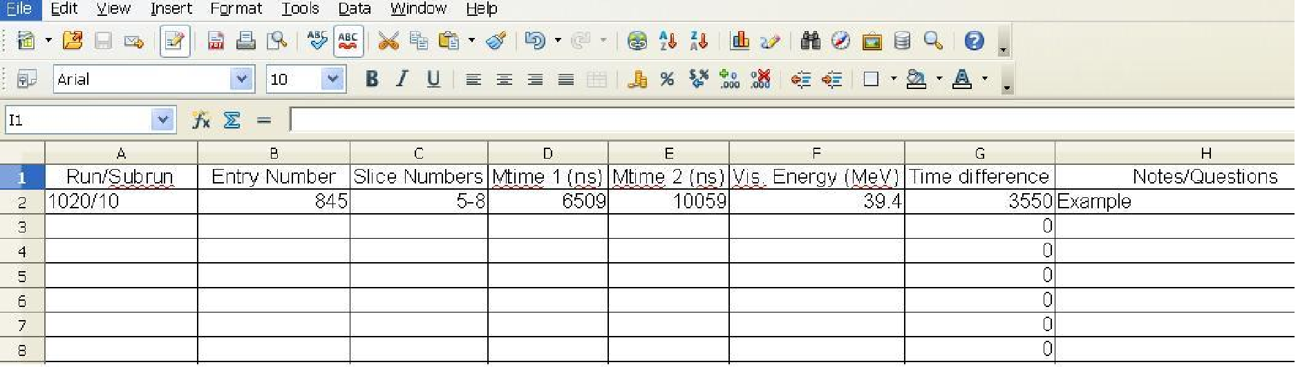
Now that we have a better idea of what muon decays look like, we will investigate a larger sample. It will become clearer that a larger sample is essential to making a more accurate measurement of the characteristic lifetime of muons. Working with your partner, you will collect data for another 15 events. This time you will record them in an Excel spreadsheet, and each student group will have a different set of data to analyze. Note: there are some minor changes from the first datasheet. This time, instead of two different slices you will just list the first slice number hyphen second slice number, MTime 1 is Mean time first slice, and MTime 2 is Mean Time second slice. Vis. Energy is Visible Energy, and this time Excel will do the subtraction for you in the Time Difference column. Look at the example included so you are familiar with the change to the data entry.
Use the list of entries your teacher has assigned for your group from the web page with all the sets of links. The List of Event Samples (Groups A through T) are found on the Particle Decay page under the category Radioactive Decay of Muons
If there are two computers available for both you and your partner, one computer can access the Arachne program, and the other can keep the Excel spreadsheet and enter data as you go. Otherwise, use the provided hard copy Excel spreadsheet, and enter the data on the computer later. The web link you use is very long and encodes the information needed to find the correct Event ID, but you will record each Event ID and can make sure you are not analyzing the same event twice. Depending on the browser you are using, you may be able to just double click on the link from the online document. When you have entered your data set and measurements into the excel spreadsheet, save it to a location and with the name designated by your teacher.
Good, you’ve got that done. Start with your set of 15 entries. Let's do some calculations on your group data set and see how they compare to the expected values for the characteristic muon lifetime. Later we will do this again for the whole class data and look at differences between the two data sets. We can again make Excel do some of the work for us. You can do this by choosing the box underneath the last value in the G column. Make sure that you are only using your own 15 entries to do this calculation. In the box enter =sum(g2:g[this will likely be somewhere around 15, more if you had any entries with multiple events]) and then enter and you will have the sum of the decay time for all the events. To find average lifetime of the muon, take the sum in your box below the last data event and divide it by the number of events.
Calculate the average lifetime of the muon decay events you found in your data, using the following equation. Nothing fancy, just the average. Remember that you may have had entries with more than one event- so count the number of events you have from your data sheet.
Average lifetime = total of all event lifetimes / number of events
= sum of numbers in column G / (row number – 1)
(If you are familiar with your spreadsheet software, there is an Average function available too.)
Now we will calculate the half-life for our data events. Lots of folks prefer to talk about half-life rather than average lifetime, but they are really the same piece of physics, just a conversion factor apart. Use the natural logarithm button on your calculator, usually written in lowercase “ln” on the calculator and by many math folks.
Half-life = Average lifetime x ln 2
This one we don't need Excel to do the work for us- just a calculator with a natural log function on it. Take the average lifetime you determined and multiple it by the natural log of 2 (which is about .693).
This simplified equation has its roots with the following expression which describes exponential decay.
If you let No be 1.0, it describes the probability that the muon will still be there after some amount of time t. Try it out with your calculator, which has an ex button. put τmean = 2.2 microseconds and try a few values for t between 0.5 and 10 microseconds and write down the answers here in the margin of this page. Don't forget the minus sign in the exponent! If you plotted the result for these different test values, what would the graph look like?
As you finish your calculations keep track of the data you collected here and compare results with other groups as they complete their data. Your teacher will be asking the class to compare your individual small group results for lifetime and half-life.
Hey, wait! We just calculated something that has a funny name. What does the half-life mean? Notice the range of time differences in your list. Some are very long, many thousands of nanoseconds. Some are quite short, just a few hundred nanoseconds. The mean lifetime is the average of those. The half-life is the amount of time after which half the muons have decayed and half have not. Compare the number you calculated to the list of time differences and see if that is approximately right. The comparison might not be exact, but it should be very close. If it is not close, double check your calculation. If it looks good after double checking your work, then congratulations! You just made a measurement of the half-life of the muon.
When all groups have completed entering their data and saving it, the next step will involve working with the whole class data set, as well as your own 15 entries. If there is wait time for other groups to complete their data entry, this is a good time to work on the follow-up questions from this round of analysis.
OK, so now you should have access to an Excel file that has the entire class data set, as well as your own group’s 15 entries. We want the larger number of events for the graphing portion of the lab. The Excel file will likely be in a read only form. Open it up, copy and paste the entire set into a new Excel document so you can modify it without messing up the original. This one you will be able to manipulate to organize data. This keeps a safe set of data available for everyone just in case there are any accidents as you manipulate the data table. Save your new one.
We are going to graph visible energy first. On the Excel spreadsheet sort your data by column F, or the visible energy data. When you choose sort, be sure that all the data in the table is highlighted. Sometimes the program does this automatically, sometimes you need to highlight everything before you choose sort from the menu. Choose ascending order on the right side. This should move all the data in order according to visible energy.
Look at the data and determine the range of data and how you will organize it on your graph. Number of events will be the y axis, and visible energy in MeV will be the x axis on your graph. Set your graph up so it occupies as much of the page as possible. You will be making a histogram graph with a bar representing the data rather than a point. You will need to set up your own range of measurements. For ease of discussion, your teacher may give you a specified range.
While someone in the class is finishing putting all of the class's data together, let's step back and think about the kind of graph we are going to make. We're going to make something called a histogram. Let's look at a histogram of some data you are more familiar with. The graph here is an example of an event histogram designed to provide a visualization of a range of occurrences of a particular type of event. This is a histogram of the number of hurricanes
which were large enough in the Atlantic Ocean to earn a name between the years of 1990 to present. Can you see a trend in the data? What can you summarize from the data as it is presented? If you had to predict the number of hurricanes in the next two years, what would your prediction be?
Okay, by now you have the whole class' data. Now make your own histogram of the energy of the events.
In preparation for constructing another graph, it helps to rearrange the data on your Excel spreadsheet to sort by time difference (column G). When you choose sort, be sure that all the data in the table is highlighted. Sometimes the program does this automatically, sometimes you need to highlight everything before you choose sort from the menu. Choose ascending order on the right side. This should move all the data in order according by time difference.
Now we will construct another graph for analysis. This one will again be a histogram showing the decay time of the muon. The data will consist of the number of events on the y axis, and time in nanoseconds on the x axis. As you set up your scales, again try to use the whole graph paper page. Your teacher may give you a set range for times (like intervals of 500 nanoseconds) to make whole class discussion and data easier.
The average lifetime of a muon is 2.2 μs (microseconds), and the measured half-life of a muon is 1.56 μs. Now we want to see how closely our whole class data matches these expected outcomes. We will repeat the process described in step 5 above, but this time using a much larger data set.
Now we will calculate the measured half-life for our data events.
Measured half-life = Average lifetime x ln 2
Like before, we don't need Excel to do the work for us- just a calculator with a natural log function on it. Take the average lifetime you determined and multiple it by the natural log of 2 (which is about .69). Actually, remember when you tried a bunch of values in your calculator using the exponential function? What value should you type in that gives an answer of exactly 0.5?
As a whole class, we will compare results and discuss why there might be differences between different sets of data, and value of making overall calculations based on a very large data set.
Questions to answer
Based on what we did in this activity, what advice would you have for someone setting up a particle interaction and decay measurement experiment? What are your recommendations about size of the experiment?
Student Chart - Note: the first 10 events are from the previous activity
Event ID | Entry Number | Slice Numbers | MTime 1 (ns) | Mtime 2 (ns) | Vis. Energy (MeV) | Time difference | Notes/Questions |
MV 2397/16/575 | 1-4 | 2385 | 5136 | 34 | 2751 |
| |
MV 2397/16/637 |
| 4-6 | 6069 | 7340 | 40.1 | 1271 |
|
MV 2397/16/845 |
| 2-8 | 4010 | 9339 | 24.3 | 5329 |
|
MV 2397/16/871 |
| 2-4 | 8823 | 10489 | 20.3 | 1666 |
|
MV 2397/16/921 |
| 4-7 | 4287 | 11164 | 30.4 | 6877 |
|
MV 2397/16/1244 |
| 3-4 | 4357 | 5840 | 25.3 | 1483 |
|
MV 2397/16/1453 |
| 2-4 | 4042 | 5117 | 58.9 | 1075 |
|
MV 2397/17/287 |
| 1-7 | 2462 | 6068 | 29 | 3606 |
|
MV 2397/17/903 |
| 6-7 | 7641 | 8770 | 15 | 1129 |
|
MV 2397/17/959 |
| 8-9 | 7979 | 10362 | 37.4 | 2383 |
|
|
|
|
|
|
|
|
|
MV 2063/1/770 |
|
|
|
|
|
|
|
MV 2063/2/574 |
|
|
|
|
|
|
|
MV 2063/2/798 |
|
|
|
|
|
|
|
MV 2063/2/856 |
|
|
|
|
|
|
|
MV 2063/2/980 |
|
|
|
|
|
|
|
MV 2063/3/970 |
|
|
|
|
|
|
|
MV 2063/4/146 |
|
|
|
|
|
|
|
MV 2063/4/840 |
|
|
|
|
|
|
|
MV 2063/4/980 |
|
|
|
|
|
|
|
MV 2063/5/346 |
|
|
|
|
|
|
|
MV 2063/5/954 |
|
|
|
|
|
|
|
MV 2063/6/128 |
|
|
|
|
|
|
|
MV 2063/6/558 |
|
|
|
|
|
|
|
MV 2063/7/322 |
|
|
|
|
|
|
|
MV 2063/8/500 |
|
|
|
|
|
|
|
|
|
|
|
|
|
|
|
MV 2063/8/534 |
|
|
|
|
|
|
|
MV 2063/8/586 |
|
|
|
|
|
|
|
MV 2063/8/696 |
|
|
|
|
|
|
|
MV 2063/8/760 |
|
|
|
|
|
|
|
MV 2063/8/888 |
|
|
|
|
|
|
|
MV 2063/9/296 |
|
|
|
|
|
|
|
MV 2063/9/308 |
|
|
|
|
|
|
|
MV 2063/9/318 |
|
|
|
|
|
|
|
MV 2063/9/626 |
|
|
|
|
|
|
|
MV 2063/10/26 |
|
|
|
|
|
|
|
MV 2063/10/118 |
|
|
|
|
|
|
|
MV 2063/10/818 |
|
|
|
|
|
|
|
MV 2063/11/180 |
|
|
|
|
|
|
|
MV 2063/11/192 |
|
|
|
|
|
|
|
MV 2063/11/906 |
|
|
|
|
|
|
|
|
|
|
|
|
|
|
|
MV 2063/12/312 |
|
|
|
|
|
|
|
MV 2063/12/834 |
|
|
|
|
|
|
|
MV 2064/1/24 |
|
|
|
|
|
|
|
MV 2064/1/34 |
|
|
|
|
|
|
|
MV 2064/1/414 |
|
|
|
|
|
|
|
MV 2064/1/782 |
|
|
|
|
|
|
|
MV 2064/1/1042 |
|
|
|
|
|
|
|
MV 2064/1/1042 |
|
|
|
|
|
|
|
MV 2064/1/1056 |
|
|
|
|
|
|
|
MV 2064/3/588 |
|
|
|
|
|
|
|
MV 2064/3/598 |
|
|
|
|
|
|
|
MV 2064/3/1046 |
|
|
|
|
|
|
|
MV 2064/4/736 |
|
|
|
|
|
|
|
MV 2064/5/190 |
|
|
|
|
|
|
|
MV 2064/5/226 |
|
|
|
|
|
|
|
MV 2064/5/380 |
|
|
|
|
|
|
|
|
|
|
|
|
|
|
|
MV 2064/5/532 |
|
|
|
|
|
|
|
MV 2064/5/918 |
|
|
|
|
|
|
|
MV 2064/5/1034 |
|
|
|
|
|
|
|
MV 2064/6/570 |
|
|
|
|
|
|
|
MV 2064/6/750 |
|
|
|
|
|
|
|
MV 2065/2/128 |
|
|
|
|
|
|
|
MV 2065/2/186 |
|
|
|
|
|
|
|
MV 2065/2/526 |
|
|
|
|
|
|
|
MV 2065/2/544 |
|
|
|
|
|
|
|
MV 2065/3/422 |
|
|
|
|
|
|
|
MV 2065/3/594 |
|
|
|
|
|
|
|
MV 2065/3/904 |
|
|
|
|
|
|
|
MV 2065/3/998 |
|
|
|
|
|
|
|
MV 2067/1/116 |
|
|
|
|
|
|
|
MV 2067/1/320 |
|
|
|
|
|
|
|
|
|
|
|
|
|
|
|
MV 2067/1/1010 |
|
|
|
|
|
|
|
MV 2067/2/154 |
|
|
|
|
|
|
|
MV 2067/2/706 |
|
|
|
|
|
|
|
MV 2067/3/84 |
|
|
|
|
|
|
|
MV 2067/3/276 |
|
|
|
|
|
|
|
MV 2067/4/740 |
|
|
|
|
|
|
|
MV 2067/4/1014 |
|
|
|
|
|
|
|
MV 2067/4/1108 |
|
|
|
|
|
|
|
MV 2067/4/1164 |
|
|
|
|
|
|
|
MV 2067/5/108 |
|
|
|
|
|
|
|
MV 2067/5/748 |
|
|
|
|
|
|
|
MV 2067/6/226 |
|
|
|
|
|
|
|
MV 2067/6/606 |
|
|
|
|
|
|
|
MV 2067/6/690 |
|
|
|
|
|
|
|
MV 2067/6/832 |
|
|
|
|
|
|
|
|
|
|
|
|
|
|
|
MV 2067/6/1060 |
|
|
|
|
|
|
|
MV 2067/7/216 |
|
|
|
|
|
|
|
MV 2067/8/788 |
|
|
|
|
|
|
|
MV 2067/68/802 |
|
|
|
|
|
|
|
MV 2067/8/924 |
|
|
|
|
|
|
|
MV 2067/8/976 |
|
|
|
|
|
|
|
MV 2067/9/86 |
|
|
|
|
|
|
|
MV 2067/9/174 |
|
|
|
|
|
|
|
MV 2067/89/220 |
|
|
|
|
|
|
|
MV 2067/9/718 |
|
|
|
|
|
|
|
MV 20679/760 |
|
|
|
|
|
|
|
MV 2067/10/146 |
|
|
|
|
|
|
|
MV 2067/10/1048 |
|
|
|
|
|
|
|
MV 2067/10/1152 |
|
|
|
|
|
|
|
MV 2067/11//90 |
|
|
|
|
|
|
|
|
|
|
|
|
|
|
|
MV 2067/11/872 |
|
|
|
|
|
|
|
MV 2067/11/896 |
|
|
|
|
|
|
|
MV 2067/11/896 |
|
|
|
|
|
|
|
MV 2067/12/92 |
|
|
|
|
|
|
|
MV 2067/12/92 |
|
|
|
|
|
|
|
MV 2067/12/322 |
|
|
|
|
|
|
|
MV 2067/13/2 |
|
|
|
|
|
|
|
MV 2067/13/268 |
|
|
|
|
|
|
|
MV 2067/13/448 |
|
|
|
|
|
|
|
MV 2067/13/490 |
|
|
|
|
|
|
|
MV 2067/13/514 |
|
|
|
|
|
|
|
MV 2067/13/826 |
|
|
|
|
|
|
|
MV 2067/14/274 |
|
|
|
|
|
|
|
MV 2067/14/448 |
|
|
|
|
|
|
|
MV 2067/14/522 |
|
|
|
|
|
|
|
MV 2067/14/1074 |
|
|
|
|
|
|
|
MV 2067/15/188 |
|
|
|
|
|
|
|
|
|
|
|
|
|
|
|
MV 2067/15/694 |
|
|
|
|
|
|
|
MV 2067/15/842 |
|
|
|
|
|
|
|
MV 2067/15/1014 |
|
|
|
|
|
|
|
MV 2067/15/1034 |
|
|
|
|
|
|
|
MV 2067/16/394 |
|
|
|
|
|
|
|
MV 2067/16/488 |
|
|
|
|
|
|
|
MV 2067/16/518 |
|
|
|
|
|
|
|
MV 2067/17/272 |
|
|
|
|
|
|
|
MV 2067/17/606 |
|
|
|
|
|
|
|
MV 2071/1/6 |
|
|
|
|
|
|
|
MV 2071/1/1004 |
|
|
|
|
|
|
|
MV 2071/2/58 |
|
|
|
|
|
|
|
MV 2071/2/498 |
|
|
|
|
|
|
|
MV 2071/3/162 |
|
|
|
|
|
|
|
MV 2071/3/258 |
|
|
|
|
|
|
|
MV 2071/3/258 |
|
|
|
|
|
|
|
|
|
|
|
|
|
|
|
MV 2071/3/818 |
|
|
|
|
|
|
|
MV 2071/3/1064 |
|
|
|
|
|
|
|
MV 2071/4/64 |
|
|
|
|
|
|
|
MV 2071/4/404 |
|
|
|
|
|
|
|
MV 2071/4/404 |
|
|
|
|
|
|
|
MV 2071/4/640 |
|
|
|
|
|
|
|
MV 2071/4/726 |
|
|
|
|
|
|
|
MV 2071/5/54/ |
|
|
|
|
|
|
|
MV 2071/5/1104 |
|
|
|
|
|
|
|
MV 2071/6/372 |
|
|
|
|
|
|
|
MV 2071/6/476 |
|
|
|
|
|
|
|
MV 2071/6/498 |
|
|
|
|
|
|
|
MV 2071/6/818 |
|
|
|
|
|
|
|
MV 2071/6/1032 |
|
|
|
|
|
|
|
MV 2071/6/1148 |
|
|
|
|
|
|
|
MV 2071/7/32 |
|
|
|
|
|
|
|
|
|
|
|
|
|
|
|
MV 2071/7/580 |
|
|
|
|
|
|
|
MV 2071/7/652 |
|
|
|
|
|
|
|
MV 2071/7/1166 |
|
|
|
|
|
|
|
MV 2071/8/894 |
|
|
|
|
|
|
|
MV 2071/8/912 |
|
|
|
|
|
|
|
MV 2071/8/1194 |
|
|
|
|
|
|
|
MV 2071/9/350 |
|
|
|
|
|
|
|
MV 2071/9/978 |
|
|
|
|
|
|
|
MV 2071/9/1136 |
|
|
|
|
|
|
|
MV 2071/10/28 |
|
|
|
|
|
|
|
MV 2071/10/412 |
|
|
|
|
|
|
|
MV 2071/11/44 |
|
|
|
|
|
|
|
MV 2071/11/44 |
|
|
|
|
|
|
|
MV 2071/11/810 |
|
|
|
|
|
|
|
MV 2071/12/156 |
|
|
|
|
|
|
|
MV 2071/12/226 |
|
|
|
|
|
|
|
|
|
|
|
|
|
|
|
MV 2071/12/268 |
|
|
|
|
|
|
|
MV 2071/12/752 |
|
|
|
|
|
|
|
MV 2071/13/310 |
|
|
|
|
|
|
|
MV 2071/13/948 |
|
|
|
|
|
|
|
MV 2071/14/204 |
|
|
|
|
|
|
|
MV 2071/14/340 |
|
|
|
|
|
|
|
MV 2071/14/942 |
|
|
|
|
|
|
|
MV 2071/14/1142 |
|
|
|
|
|
|
|
MV 2071/15/766 |
|
|
|
|
|
|
|
MV 2071/15/808 |
|
|
|
|
|
|
|
MV 2071/15/852 |
|
|
|
|
|
|
|
MV 2071/15/884 |
|
|
|
|
|
|
|
MV 2071/15/1034 |
|
|
|
|
|
|
|
MV 2071/16/172 |
|
|
|
|
|
|
|
MV 2071/16/258 |
|
|
|
|
|
|
|
|
|
|
|
|
|
|
|
MV 2071/16/388 |
|
|
|
|
|
|
|
MV 2071/16/440 |
|
|
|
|
|
|
|
MV 2071/16/1028 |
|
|
|
|
|
|
|
MV 2071/16/1036 |
|
|
|
|
|
|
|
MV 2071/17/746 |
|
|
|
|
|
|
|
MV 2071/17/950 |
|
|
|
|
|
|
|
MV 2071/18/16 |
|
|
|
|
|
|
|
MV 2071/18/412 |
|
|
|
|
|
|
|
MV 2071/18/952 |
|
|
|
|
|
|
|
MV 2071/20/304 |
|
|
|
|
|
|
|
MV 2071/20/402 |
|
|
|
|
|
|
|
MV 2071/20/458 |
|
|
|
|
|
|
|
MV 2071/20/702 |
|
|
|
|
|
|
|
MV 2071/20/764 |
|
|
|
|
|
|
|
MV 2071/21/208 |
|
|
|
|
|
|
|
MV 2071/21/208 |
|
|
|
|
|
|
|
|
|
|
|
|
|
|
|
MV 2071/21/634 |
|
|
|
|
|
|
|
MV 2071/22/116 |
|
|
|
|
|
|
|
MV 2071/22/116 |
|
|
|
|
|
|
|
MV 2071/22/494 |
|
|
|
|
|
|
|
MV 2071/22/804 |
|
|
|
|
|
|
|
MV 2071/23/618 |
|
|
|
|
|
|
|
MV 2071/23/586 |
|
|
|
|
|
|
|
MV 2071/24/714 |
|
|
|
|
|
|
|
MV 2071/25/276 |
|
|
|
|
|
|
|
MV 2071/25/680 |
|
|
|
|
|
|
|
MV 2071/26/382 |
|
|
|
|
|
|
|
MV 2071/26/886 |
|
|
|
|
|
|
|
MV 2072/2/878 |
|
|
|
|
|
|
|
MV 2072/2/1042 |
|
|
|
|
|
|
|
MV 2072/2/1178 |
|
|
|
|
|
|
|
MV 2072/3/118 |
|
|
|
|
|
|
|
|
|
|
|
|
|
|
|
MV 2072/3/238 |
|
|
|
|
|
|
|
MV 2072/3/306 |
|
|
|
|
|
|
|
MV 2072/3/426 |
|
|
|
|
|
|
|
MV 2072/3/580 |
|
|
|
|
|
|
|
MV 2072/3/922 |
|
|
|
|
|
|
|
MV 2072/4/582 |
|
|
|
|
|
|
|
MV 2072/4/582 |
|
|
|
|
|
|
|
MV 2072/4/624 |
|
|
|
|
|
|
|
MV 2072/5/336 |
|
|
|
|
|
|
|
MV 2072/5/734 |
|
|
|
|
|
|
|
MV 2072/5/1056 |
|
|
|
|
|
|
|
MV 2072/6/108 |
|
|
|
|
|
|
|
MV 2072/6/330 |
|
|
|
|
|
|
|
MV 2072/7/834 |
|
|
|
|
|
|
|
MV 2072/8/114 |
|
|
|
|
|
|
|
MV 2072/8/608 |
|
|
|
|
|
|
|
|
|
|
|
|
|
|
|
MV 2072/8/848 |
|
|
|
|
|
|
|
MV 2072/8/944 |
|
|
|
|
|
|
|
MV 2072/8/944 |
|
|
|
|
|
|
|
MV 2072/9/712 |
|
|
|
|
|
|
|
MV 2072/9/1014 |
|
|
|
|
|
|
|
MV 2072/9/1180 |
|
|
|
|
|
|
|
MV 2072/10/212 |
|
|
|
|
|
|
|
MV 2072/10/212 |
|
|
|
|
|
|
|
MV 2072/10/572 |
|
|
|
|
|
|
|
MV 2072/10/698 |
|
|
|
|
|
|
|
MV 2072/11/352 |
|
|
|
|
|
|
|
MV 2072/11/416 |
|
|
|
|
|
|
|
MV 2072/11/818 |
|
|
|
|
|
|
|
MV 2072/11/1020 |
|
|
|
|
|
|
|
MV 2072/11/1096 |
|
|
|
|
|
|
|
MV 2072/12/224 |
|
|
|
|
|
|
|
MV 2072/13/678 |
|
|
|
|
|
|
|
This is the suggested fourth activity in the muon radioactive decay lessons.
This is an advanced activity, suitable if you have a lot of time or have one or two students interested in a little more. But it has a compelling and historical detective story. The student instructions lead them and you through the argument through a process of elimination. Here are a few additional notes.
Goals:
Prior Knowledge:
Materials:
Notes for the teacher:
The arguments that are central to this activity are by themselves simple, but to reach the conclusion requires stringing them together and considering specific consequences of the situation, not just general principles. This is a rewarding challenge, and you may want to allow your students plenty of time to think things through and talk out loud with their partners. As Sherlock Holmes said, “When you have eliminated the impossible, whatever remains, however improbable, must be the truth”. This is one of those situations.
Notice in the suggested answers that we are making semi-quantitative arguments. Lots of students have a great resistance to this, but if you hear them stepping toward a correct answer, consider challenging them with the question “what are the consequences of your argument if your electron has this energy” and point somewhere in their histogram. See how they respond.
Answers to the student activity questions:
Option one. Suppose that only one particle, the electron, came out. Given the energy available and the kinetic energies in the histogram, do you notice something odd? Thinking about an electron moving with any of those kinetic energies what do you conclude about conservation of momentum?
Answer. The electron must have all 106 MeV of kinetic energy, but clearly that is not what I measured, I usually only saw half of that. And if the electron is the only particle, and it has that much kinetic energy, it must have some momentum, because even if it has 30 MeV, it really is moving, right? But there was no momentum before (muon at rest), so having momentum after would violate a conservation law, which I would never do, officer, really. This situation not only does not describe the electrons I measured, but it's physically impossible.
Option two. Suppose that two particles came out: the electron that you can see, and a neutrino or neutrissimo or something which you don’t see. To simplify the argument for a second, enough that you can do the math in your head, pretend these two particles have equal mass, like billiard balls. Consider conservation of momentum, what must be the direction of the neutral particle you didn’t see, relative to the electron you did see? Given the available energy, what must be the kinetic energy of each of these two particles? If that was really how it worked, what would your energy histogram have looked like? [This conclusion stands even if the masses of the two particles are different, it just requires a more difficult calculation to figure out what energy would have been in the.]
Answer: This one is tricky, but if I assume both particles have the same mass, it really is easier. In this case, they must come out back to back (so 2D vector momentum sums to zero and is conserved). If that happens, and they have the same mass, then they also have the same momentum and must have equally shared the available energy, and have 53 MeV each. In this case, ALL the electrons should have 53 MeV, they all would be piled up in 50 to 55 MeV interval in the histogram. That’s clearly not what I see.
Longer answer: If the masses of the electron and neutrino were different, they would still be piled up in just one interval in the histogram, they would still come out back-to-back, but which one (between 0 and 106) depends on what the two masses are. Mathematically, you set up conservation of energy, conservation of momentum, and get two equations and two unknowns, which has exactly one solution.
Option three. Supposed three particles came out. How does this situation change or overcome the issues you wrestled with for the previous two options.
Answer: I certainly don’t have the problem I had in option one, I have three particles to share the energy and conserve momentum. The three particles don’t have to come out perfectly back to back anymore; in fact I can imagine all sorts of combinations of directions that still balance momentum. If I give the electron only 20 MeV of energy, then I just give the neutrinos the other 86, and make sure they make a wide enough angle from each other, centered on a line backward from the electron. Change the electron energy higher; make the angle between the two neutrinos smaller. [It is not super clear from this qualitative argument that the limiting case is that the electron can carry at most half the available energy, like the argument in option two, but this is also true.]
Summarize as succinctly as you can summarize the process of elimination that leads from your histogram to your conclusion that there must be at least two unseen particles with the electron after the decay.
Having only one particle after the decay is impossible; no way can it conserve energy and momentum. Having two particles is possible, but then I would expect a single energy somewhere between zero and 106 MeV, but instead I see a range of energies. Having eliminated the two simplest possibilities, I can imagine that having three particles will work; they give me lots of ways to conserve both momentum and energy. Now I see that the electron gets energy between zero and about 60 MeV, and the two neutrinos share the rest and go off unseen but in directions that allow them to conserve momentum.
Instructions for students:
Here we invokes conservation of energy and conservation of momentum to deduce (as it was understood historically) that the electron from the decay must be accompanied by at least two neutrinos, not one and not zero, even though we did not see or measure either of the neutrinos.
In the previous activity, you recorded the energy of the electron in each decay. At the time, it was primarily so that you can confirm that it was less than 60 MeV, because larger values mean you were about to be fooled into picking the wrong slice for your decay electron. Both of those energies tell their own interesting story. Choose some intervals and on your graph paper make a histogram of the energies (column F) of your data. It should look something like this.
Looks like some shape, kind of a bell curve, but maybe not really. But this shape has a surprising piece of information in it.
The muons you observed slowed down and came to a stop in the detector. You know this was probably true, because you saw electrons coming out in all directions. If the muon hadn’t stopped, and still had momentum, the electrons would have carried some of that momentum. Great, the muon was at rest with zero momentum.
The other important feature is that we have a very specific amount of kinetic energy we can work with. The 106 MeV rest energy (mass) of the muon that was converted into the tiny masses of the electron and neutrinos. All this energy must be present, but we will consider how it can and cannot be shared among the different particles.
Consider the following options for the decay.
Option one. Suppose that only one particle, the electron, came out. Given the energy available and the kinetic energies in the histogram, do you notice something odd? Thinking about an electron moving with any of those kinetic energies what do you conclude about conservation of momentum?
Option two. Suppose that two particles came out, the electron which you can see, and a neutrino or something which you don’t see. To simplify the argument for a second, enough that you can do the math in your head, pretend these two particles have equal mass, like billiard balls. Consider conservation of momentum, what must be the direction of the neutral particle you didn’t see, relative to the electron you did see? Given the available energy, what must be the kinetic energy of each of these two particles? If that was really how it worked, what would your energy histogram have looked like? [This conclusion stands even if the masses of the two particles are different, it just requires a more difficult calculation to figure out what energy would have been in the.]
Option three. Supposed three particles came out. How does this situation change or overcome the issues you wrestled with for the previous two options.
Summarize as succinctly as you can summarize the process of elimination that leads from your histogram to your conclusion that there must be at least two unseen particles with the electron after the decay.
Goal:
This quick quiz is meant to be used after viewing the What is MINERvA? - PowerPoint (found in the activities section of the website). The quiz is located at the end of the presentation but is given here in case the teacher would prefer a printed copy.
Quiz
MINERvA
(Main INjector ExpeRiment) for v-A
1. What does the MINERvA detector measure?
2. What shape is each of the planes in MINERvA?
3. What is a scintillator strip?
4. What is the shape of a scintillator strip?
5. How many specialized areas are in MINERvA?
6. Name 3 types of material in MINERvA.
7. What is a wavelength shifting fiber?
8. What does a PMT do?
ANSWER KEY
1. What does the MINERvA detector measure?
It measures low energy neutrino interactions (interactions of protons, muons and pions in particular)
2. What shape is each of the planes in MINERvA?
Each plane is in the shape of a hexagon.
3. What is a scintillator strip?
It is a material that takes the energy from an interacting particle and turns it into light.
4. What is the shape of a scintillator strip?
Triangular shaped and come in long strips.
5. How many specialized areas are in MINERvA?
There are three areas: The fully active target, the ECAL and the HCAL.
6. Name 3 types of material in MINERvA.
Currently the detector has specialized areas made out of hydrocarbon, carbon, iron and lead. There are plans to add helium and water targets in the near future.
7. What is a wavelength shifting fiber?
It takes the light and collects it and sends it to the PMT’s. (It also shifts the wavelength of the light to better collect it.)
8. What does a PMT do?
The signal from the detector will be a very weak signal. The computers are not able to read neither the minute strength of the signal nor do they recognize the photons that they are receiving from the detector. The PMT takes the photons and amplifies the signal. It also transfers the signal into a form of energy which is more easily understood by the computers.
Goal:
To construct a 3-dimensional, simplified model of the MINERvA apparatus for classroom reference and discussion with emphasis on momentum conservation
Prior Knowledge:
A basic knowledge of what MINERvA is from viewing the ‘What is MINERvA? - PowerPoint’ found in the Classroom Activities section of the website
Materials:
20 - Paper card-stock hexagons (Optional: use 3 different colors of cardstock, having a combination of 10, 5, and 5 for the hexagons)
Hole puncher
Scissors
3-different colored pipe cleaner
8 inch dowel
Glue
Tiny puffy-balls
Directions for Students:
Inner Strips upright (center)
Inner Strips 60º right of center (right diagonal)
Inner Strips upright (center)
Inner Strips 60º left of center (left diagonal)
(Repeat the above pattern with the remaining hexagons)
Note: you may want to glue the hexagons back to back so that you can see the directionality of the rods
If needed, glue the modules in place on the dowel after the model is completely constructed.
To demonstrate the possibility of muon decay, the short pipe-cleaner should travel to the 8th module. On the 10th module glue a puffy ball to represent the “Michel” electron produced in the decay.
NOTE: The neutron will not produce both types of muons (one that decays and one that travels through the active target area) at the same time. These would be 2 separate events; representing 2 possible outcomes for the muon based on its energy level.
Diagram:
Analysis Questions:
__________________________________________________________________
__________________________________________________________________
__________________________________________________________________
__________________________________________________________________
____________________________________________________________________
____________________________________________________________________
____________________________________________________________________
____________________________________________________________________
This teacher-guided activity is the first suggested activity in learning about scattering of neutrinos and applying conservation of momentum.
Goal:
In this teacher-guided activity, students will be introduced to the concept of conservation of momentum and energy at the particle level.
Teacher Background:
Before starting this activity, students should have already gone through the ‘Directions for the Simple Arachne Website’ since they will have a have a level of comfort within the website and the information they need to record about the interaction.
Another resource to view prior to this activity is the ‘Bug and Truck Collision’ PowerPoint (found on the main website, “Momentum conservation” page and under the “Activities and Resources"). The PowerPoint provides a humorous visual representation of the collision and its products. To access the data, be sure that the student computers have Firefox installed for internet usage. The Arachne website will not work on Internet Explorer
After reviewing the Student Background information with the class, teachers will guide the students through several examples of collisions. Have the students open the first collision. Guide them to highlight either the shorter or longer track. The longer track will be the path of the muon and the shorter track will be the path of the heavier proton. When they hold the cursor over one of the tracks the color will change to red. A drop-down box will appear. Make sure they choose the correct particle information for the path they have selected and record it on their collection sheet. (You will also notice the ‘Copy’ box. If you prefer, students can have the information copied and pasted into an excel file instead of using the Collection sheet provided) Repeat the same procedure for the other path. It is very important that they write down the negative sign if it appears next to the momentum values. If you choose you can guide the students through the first few events and then let them try the remainder in small groups.
After the students have recorded data from 10 events, the sum of the values should be calculated. Students will find that the sum of the px and the sum of the py do not equal zero. This will lend itself to the discussion of ‘Is the neutron at rest inside the nucleus?’ You may want to refer back to the ‘Bug and Truck Collision’ PowerPoint for visual explanation.
Based on the explanation below in the Background Information-MINERvA Reaction the KE + 104 MeV will tell the students the original energy of the neutrino prior to its collision with the neutron.
Focusing on using actual data from the MINERvA experiment at Fermilab to apply the law of conservation of momentum to neutrino collisions with atomic neutrons, the equation that sums up the reaction that are being detected:
υμ- + n0→ p+ + μ-
The equation shows that when a high-energy neutrino (υμ-) scatters off a neutron (n0) in the nucleus of a carbon atom, one result can be the production of a proton (p+) and a muon (μ-). The detectors in MINERvA can precisely record the momentum & kinetic energy of the products (proton & muon); and by applying the law of conservation of momentum to this information one can readily determine the momentum & KE of both the incoming neutrino and the “stationary” neutron in the nucleus of the carbon atom. One important student outcome is the ability to determine that neutrons in a nucleus are hardly stationary – the calculated momenta of the neutrons will show a significant non-zero distribution.
Instructions for Students -MINERvA’s reaction:
Since the laws of conservation and momentum must be obeyed, it is possible to use the data collected to determine the energy of the incoming neutrino and if there was neutron momentum prior to collision.
To access the data, one must become familiar with the data filtering website, Simple Arachne (More details on how to use Arachne can be found in the Directions for Simple Arachne within this teacher’s guide). The Arachne webpage contains a wealth of information about individual neutrino scattering events, of which students will record only a small portion. The basic steps are as follows:
1. Click on link to pre-chosen neutrino scattering event. This leads to page w/ relevant info.
2. Record ENTRY # & SLICE # of the event (located in top left corner)
3. Locate the Big Hitmap in the center of page. There you will see a branching track showing the proton and muon (each moving w/ their respective KE & momentum)
4. Mouse over to either particle track to magnify it. The long, straight track is the muon and the short, angled track is the proton.
5. While a track is magnified, click on it & information about each particle’s KE & momentum will appear to the right. Choose the correct particle data (that matches the track you've highlighted) and record relevant data (px, py & pz) .
6. Note: the default units for momentum are MeV/c. If desired, you can easily switch to SI units by clicking the button.
7. Once information on 1st particle (say the proton) is recorded, then go back and mouse over the track of the other particle (muon), click, and record relevant information.
The following information needs to be recorded for both the proton and muon:
px and py: These values are added together and should sum up to zero if the neutron was at rest prior to the collision. If they don't add to zero, then the neutron must have had some initial momentum in those directions (it's jiggling around in the nucleus)
pz: This is the momentum along the beam axis. The momentum of p+ + μ- along the z-axis should equal that of the original neutrino since it entered the nucleus along the z-axis.
Each lab group should record data for the same 10 neutrino/neutron collisions to realize that there is a distribution of momenta for both the neutrino and atomic neutron.
Steps 1 and 2:
Step 3:
Steps 4 and 5:
Step 7:
Conservation of Momentum Events
Events are posted at http://neutrino-classroom.org/momentum_conservation.html#collisions in groups of 20 per group.
Note: Arachne requires a recent version of a web browser, such as Firefox version 4.0, Safari version 4.0, and Chrome version 5.0. Arachne relies on Java and parts of the HTML5 standard to more dynamically render the images and make them interactive. Because it does not yet support the latter, the Internet Explorer browser will not run Arachne.
muon | proton | muon + proton total | ||||||||||||||
KE | v | px | py | pz | KE | v | px | py | pz | ΣKE | Σpx | Σpy | Σpz | |||
entry | (MeV) | c | (MeV/c) | (MeV/c) | (MeV/c) | (MeV) | c | (MeV/c) | (MeV/c) | (MeV/c) | (MeV) | (MeV/c) | (MeV/c) | (MeV/c) | ||
Questions
1. Determine the smallest and greatest sum in momentum along the z-axis.
2. How many of the sum of px and sum of py are positive and how many are negative?
3. Why are the z-axis momenta always so much larger than either the x or y-axis momenta?
4. Before the collision what was assumed about the momentum of the neutron along the x & y-axis?
5. Looking at the sum in momentum along the x & y-axis what must one now conclude about the initial momentum of the neutron? Justify.
Example form:
muon | proton | muon + proton total | ||||||||||||||
KE | v | px | py | pz | KE | v | px | py | pz | ΣKE | Σpx | Σpy | Σpz | |||
entry | (MeV) | c | (MeV/c) | (MeV/c) | (MeV/c) | (MeV) | c | (MeV/c) | (MeV/c) | (MeV/c) | (MeV) | (MeV/c) | (MeV/c) | (MeV/c) | ||
268 | 7347 | 1.0 | 340 | -394 | 7433 | 184 | 0.5 | -394 | 216 | 422 | 7531 | 54 | 178 | 7854 | ||
866 | 3712 | 1.0 | -7 | -502 | 3783 | 159 | 0.5 | 279 | 74 | 490 | 3871 | 272 | 428 | 4273 | ||
271 | 998 | 1.0 | 200 | 149 | 1069 | 290 | 0.6 | -473 | 31 | 635 | 1287 | 273 | 181 | 1703 | ||
362 | 1162 | 1.0 | -207 | -225 | 1225 | 351 | 0.7 | 364 | 171 | 787 | 1513 | 157 | 55 | 2012 | ||
338 | 1296 | 1.0 | -135 | 273 | 1363 | 362 | 0.7 | 32 | -587 | 681 | 1658 | 103 | 314 | 2044 | ||
In this self-guided activity, students will analyze more neutrino interactions using conservation of momentum, and will infer properties of the target neutron inside a carbon nucleus.
Teacher’s Guide:
MINERvA Billiard Ball Reaction
Intermediate Level
Goals:
Notes of the Teacher
This activity asks your students to use conservation of momentum to investigate a two particle collision between a fast moving neutrino (υμ-) and a “stationary” neutron (n0). Stationary is in quotes because neutrons actually vibrate and zip around the confines of an atom’s nucleus at surprisingly high speeds. A proton and a muon are the particles produced in this collision. The particle collision is represented below:
υμ- + n0→ p+ + μ- |
MINERA provides information about each product particles momentum and energy. Students will focus on the product momenta data to:
This intermediate activity adds a layer of complexity to data analysis because separate student results must be merged together and then presented to the class. Merging can be done by hand with students in the classroom or by the teacher merging student Excel files.
Prerequisite Knowledge:
Incorporating Excel:
This activity gives you the option to let your students use Excel to organize, manipulate and display data. The Arachne site is compatible with Excel. Instead of students writing down muon and proton data on a worksheet and then adding the data and graphing it by hand, the computer quickly transfers event data from Arachne to Excel with the click of a few buttons. Then, the students can use Excel formulas to add the data.
When students are comfortable determining if the track information describes the muon or the proton, the next step is to COPY the information into Excel. This is done in three steps
An Excel template is provided on the website under the resources for the momentum conservation exercise. This template is useful because it gives a uniform data collection sheet for all students. When students open this template they will see a screen that looks like the screen shot below.
Before a student copies data from Arachne into Excel, the entry file number that appears on the left hand side of the Arachne screen should be typed into Excel’s cell A3 under the heading “event”.
Students should copy data from their first Arachne entry file into row 3. Specifically, muon data is pasted into cells B3 through F3. Proton data is pasted into cells H3 through L3.
The paste command works if students click on cell B3 for muon data and cell H3 for proton data. For the second Arachne entry file, data is pasted into cells B4 and H4. Data from the third Arachne entry file is pasted into cells B5 and H5, etc. Muon and proton data from the 10th Arachne entry file appear in row 12.
As the students type, the command will appear in Excel’s cell N3 and look like the snapshot below.
Cell N3 is now populated by the sum of the KE’s that appear in cells B3 and H3
--------------------------------------------------------------------------------------------------------------------
Cell O3 will be populated with the sum of cell D3 and J3.
---------------------------------------------------------------------------------------------------------------------
The command to sum the y-axis momenta in cell P3 is: =E3+K3
The command to sum the z-axis momenta in cell Q3 is: =F3+L3
Student data runs for analysis:
Use the list of entries your teacher has assigned for your group from the web page with all the sets of links. List of entries (grouped A through T) are found on the web page under the Momentum Conservation tab: Analyzing Neutrino Collisions
Merging Data:
After students have completed their Excel template, the data can be merged using the ‘Merging Excel Spreadsheets from Student Groups’ section of this Teacher Guide
Goals
A fun activity that uses a ‘Standard Model of Fundamental Particle and Interactions’ chart that sends students looking around for the answers. This chart can be found on the internet and in many classrooms
Your will need these materials
Notes for Teachers
This activity is designed to be a quick ‘prior-knowledge activity’ so that students become familiar with the vocabulary associated with particle physics
Student Instructions and activity sheet
Standard Model Scavenger Hunt – Using a Standard Model of Fundamental particle and Interactions chart, complete the following questions:
Goals:
A little bit of fun looking at the variety of neutrino interactions visible in the MINERvA data.
You will need these materials:
1. Website access to Arachne and this web page with links to many events.
2. Excel data sheet (available for download here)
3. Calculators
4. Graph paper for drawing a graph
5. Page of follow-up questions
Notes for the teacher:
This is an optional activity to provide a little more depth to the MINERvA experiment.
After you have worked with students through the first two Arachne activities, you can have your students look at some other types of particle interactions beyond the muon decay events that were emphasized in the earlier activities. The Particle Scavenger Hunt makes use of the ability to maneuver around in Arachne to view any event you like, by just changing the entry number after you have accessed a particular run/subrun set. In this activity students are encouraged to explore and find examples of a number of different types of events. You could choose to wait to show the students the Types of Events PowerPoint until you reach this point, or if you have already shown it to the students, they could access it on their own to refresh themselves about the other types of events that can be found.
This is a great way to take a bigger picture look at what the MINERvA experiment is providing for the world of particle physics. For example the events don't always start at the front of the detector. How could this happen? Well, perhaps a particle that has no charge (such as neutron) enters the detector and then begins the decay process and produces a charged particle or particles that are then detectable- and these particles may also decay into other particles in the detector. See the background information below for examples of the many possibilities that can happen. After some exploration on their own, students should begin to see some of the different possibilities beyond muon decay- they may not be able to identify what is happening, but they should be able to recognize these events as different from what they saw in the muon decay activities.
Particle Scavenger Hunt Student Instructions and activity sheet:
Here is a fun activity to try. Find the following types of events in the Arachne Database. If you need to, refer back to the Types of Events PowerPoint. In the blank beside its description, write down the information for the specific event. You can maneuver in Arachne by pressing the “Next Gate” or “Previous Gate” buttons. You can see these buttons circled in the diagram to the right.
Find the following types of events:
Description of Event | Run/Subrun | Entry | Slice(s) | |
A track going all the way through |
|
|
| |
More than one track in one slice |
|
|
| |
At least 3 tracks |
|
|
| |
Two tracks that meet at a spot in the middle of the detector |
|
|
| |
A slice where three or more tracks come from the same point. |
|
|
| |
A particle enters from the top or bottom of the detector |
|
|
| |
A track that stops in the detector |
|
|
| |
A track that begins in the ECAL |
|
|
| |
A track that begins in the HCAL |
|
|
| |
A small splashy event |
|
|
| |
A large splashy event |
|
|
| |
An electron being emitted in the "backwards" direction |
|
|
| |
Three more muon / electron events that have not been listed |
|
|
| |
|
|
|
| |
|
|
|
| |
A short burst of energy |
|
|
|
Now, here is the fun part – this is a competition to all who do this activity. Find the following events:
Description of Event | How Much/Many | Run/Subrun | Entry | Slice(s) |
Find the slice with the most Visible Energy |
|
|
|
|
Find an electron with the most Visible Energy |
|
|
|
|
Find an event with the most tracks |
|
|
|
|
The gate with the most slices |
|
|
|
|
Here is the final challenge. Find interesting events and use your own judgement to determine what might be happening in these events.
Your Description of Event | Run/Subrun | Entry | Slice(s) |
|
|
|
|
|
|
|
|
|
|
|
|
|
|
|
|
The following information may be useful in your understanding of particle physics. It discusses a few issues that are reasonable questions that you or the students may have, but are not actually needed for doing the activities.
Creating a neutrino beam: how do they do it at Fermilab and why does it work?
Rules govern particle decay and particle collisions (interactions), each of which are or are related to a conservation law, and require equal amounts of something to be present on both sides of a reaction equation. All of these rules must be followed in every decay/interaction! The examples below are primarily reactions that produce neutrinos or govern neutrino interactions in MINERvA, but you will see or remember the rules applied to muon decay as well.
Charge must be conserved -- equal on both sides. For example if the net charge on the left is negative one, there must also be a net charge of negative one on the right side.
Flavors must be conserved- if there is a representative from the muon family on one side there must also be a muon flavor member of the other side. This can take the form of muon one side and muon neutrino on the other side.
When counting how many muon-flavors there are, a muon has +1 but an anti-muon has -1. In effect, if you have a muon and an anti-muon-neutrino on the same side you have (+1) + (-1) = 0 muon flavor total. Same with electron flavor and you’ll remember muon decay has an electron and an anti-electron neutrino on one side, for zero total electron flavor.
The number of nucleons (protons or neutrons, doesn’t matter what mixture) on one side must have a corresponding equal number of nucleons on the other side. If there are a proton and a neutron on one side, there must be two nucleons on the other side, often which ones is determined along with the need to conserve charge.
Most importantly, energy and momentum must be conserved. But, totally cool, you can see Einstein's relativity expression E=mc2 in play in these reactions, we can turn mass into energy and vice versa!
So how do you take those rules and use them to get a beam of muon neutrinos for the MINOS and MINERvA experiments? Well, it takes some very large scale stuff to make these incredibly small particles. Start with hydrogen gas, carrying one proton and one electron, right? Strip off the electron, and you have basically just a positively charged proton running around. Speed it all up along with a bazillion other protons to almost the speed of light, and then slam the protons into a carbon target where they hit protons or neutrons of carbon atoms. At this point if a proton hits another proton the result will be a positive pion and a proton and a neutron. If a proton hits a neutron instead you will get either a positive or negative pion and two protons or two neutrons. Possibilities sketched out below.
p+ + p+ → π+ + p+ + n0
proton + proton → pion + proton + neutron or
p+ + p+ → π0 + p+ + p+
proton + proton → neutral pion+ proton + proton or
p+ + n0 → π+ + n0 + n0
proton + neutron → pion + neutron + neutron
p+ + n0 → π0 + p+ + n0
proton + neutron → neutral pion + proton + neutron
p+ + n0 → π- + p+ + p+
proton + neutron → pion + proton + proton
This produces a stream of interesting sub-atomics particles called pions which are charged and heading toward our detector. But we want neutrinos, not pions! Hmm. These are all unstable and have relatively short lifetimes 26 ns for pions. When these particles decay they almost always (99% of the time) decay to a positively charged muon plus muon-neutrino pair. (There is another process where a different particle called a kaon is produced which often decays to electrons, which isn’t so important for this particular story.)
Only two variations are listed.
π- → μ- + anti-νμ
pion → muon + anti-muon neutrino
π+ → μ+ + νμ
pion → anti-muon + muon neutrino
Writing it this way visually emphasizes the muon and its neutrino are sibling pairs of particles. And they come in particle and anti-particle forms. Now we have neutrinos heading toward our detector. In the detector they interact with whatever the detector is made of. There are lots and lots and lots of interesting ways this interaction can happen; one simple interaction is this:
anti-νμ + p+ → n0 + μ+
anti-muon neutrino + proton → neutron + anti-muon
νμ + n0 → p+ + μ-
muon neutrino + neutron → proton + muon
There is an exercise here that looks at the variety of things that come out of the neutrino interaction with nuclei in the detector. This is one of the fun things we can see in the MINERvA neutrino data. These behave like a classic billiard ball collision you see in your physics textbook, and is how we “see” neutrinos.
There is also exercise that looks at the resulting muons which decay in the detector. The latter involves the anti-muon there on the right hand side above, and is another thing that is fun to see in the MINERvA data.
The anti-muon is fun to look at, because unlike the above, we can watch this one decay using the MINERvA detector. Its decay is like this.
μ+ → e+ + νe + anti-νμ
anti-muon → positron + electron neutrino + anti-muon neutrino
Wow! We will only be able to see the positron, and interesting, even more neutrinos!
(If you are interested, you notice we followed the negative pion to the anti-muon neutrino to an anti-muon to a positron. Not fully shown here, we can follow the positive pion to the muon neutrino to the negatively charged muon to a negative electron. This is fun too, but negative muons don’t always decay, sometimes they are captured by an atom almost as if they were an electron. But then they often get sucked into the nucleus before they decay, so that’s why we’re not going to concentrate on those.)
.
Open Excel Sheets to Merge - First open Excel. Open the spreadsheets that have the same headers. Now you want to put all of this information in the same spreadsheet. Create a new spreadsheet by clicking the 'new' icon at the top.
Merge the Separate Spreadsheets - Now go up to 'data' and choose 'consolidate.' A window will open. Choose 'sum' as the function under the drop down menu. Now for the references, click the 'browse' button. Go up to window and choose your first spreadsheet. Click and drag an area with your information in it. Leave lots of room at the bottom. Now click the icon in the consolidation window and then click 'add.' Do the same with your other spreadsheets.
Automatically Update the Merge Spreadsheet - The spreadsheets all have the same headers, so check off 'Use Labels in Top Row and Left Column.' If you plan on changing your data in their individual files, you can check this box so the merged spreadsheet will automatically update when you open it again. Click 'ok.'
Teacher Background Information for Introducing Histograms to Students
The following lessons and worksheets were designed to provide a basic format when introducing the concept of data collection and histograms (bar graphs of frequency) to students. The following are explanations to the lessons.
Histogram Worksheet –
This worksheet is designed to introduce the students to Histograms. It can be used at any time but may serve as a good spring board as to what a histogram is and how it is useful in data analysis.
Histograms and Distribution (hands on) –
This activity is designed as a hands-on demonstration of how ‘random’ distributions of paper punch-outs fall on a grid. Questions are posed to the student at the end of the activity and a teacher answer sheet is included to help facilitate the discussion.
Note: The activity is designed to be done in the classroom; however, a variation can be done outside on a football field with students throwing balls from each end zone toward center field
Histograms Lesson 1 –
This lesson takes ‘canned data’ from rolling a ball down a ramp and has the students determine groupings (bins), sorting the data into the bins and graphing by hand the results of the sorting. Questions are posed to the student at the end of the activity and a teacher answer sheet is included to help facilitate the discussion.
Histogram Worksheet
The 3 histograms below show the batting averages of the winners of the batting title in the major league baseball (for both the American & National leagues) for certain years in the 1900s. Batting average shows the percent (written as a decimal) of the time a certain player gets a hit. A player who has a batting average of 0.405 has gotten a hit in 40.5 % of the times that they were at bat. The batting title is an award given to the player with the highest batting average for a given season. Refer to the histograms as you answer questions 1 – 6.
_________1. How many batting titles were won with a batting average of between 0.300 and 0.350 from 1901 to 1930?
_________2. How many batting titles were won with a batting average of between 0.300 and 0.350 from 1931 to 1960?
_________3. How many batting titles were won with a batting average of between 0.300 and 0.350 from 1961 to 1990?
4. If you were to find the mean of each of the winning batting averages for each time period, which time period do you think would have the highest mean? Explain.
____________________________________________________________________________________________________________________________________________________________________
5. As the century progressed, what in general happened to the batting averages of the batting title winners? Explain.
____________________________________________________________________________________________________________________________________________________________________
____________________________________________________________________________________________________________________________________________________________________
For questions 6 – 10, refer to the following 2 histograms. These histograms were made in an attempt to determine if William Shakespeare was really just a pen name for Sir Francis Bacon. (A pen name is a fake name used by another person when writing). A few scholars have had this idea and in order to determine if this was true, a researcher had to count the letters in every word of Shakespeare’s plays & Bacon’s writing (and you thought you had a lot of homework). Their results are recorded in the histograms below.
_________6. What percent of all Shakespeare’s words are 4 letters long?
_________7. What percent of all Bacon’s words are 4 letters long?
_________8. What percent of all Shakespeare’s words are more than 5 letters long?
_________9. What percent of all Bacon’s words are more than 5 letters long?
10. Based on these histograms, do you think that William Shakespeare was really just a pen name for Sir Francis Bacon? Explain.
_____________________________________________________________________________________________________________________________________________________________________________________________________________________
Suppose that the two histograms above show the sleeping habits of the teens at two different high schools. Wheatland High School is a small rural school consisting of 100 students while Urbandale High School is located in a large city and has 3,500 students.
_________11. About what percent of the students at Wheatland get at least 8 hours of sleep per night?
_________12. About what percent of the students at Urbandale get at least 8 hours of sleep per night?
_________13. Which high school has more actual students that sleep between 9 – 10 hours per night?
_________14. Which high school has a higher median sleep time?
15. Wheatland’s percent of students who sleep between 8-9 hours a night is ________ % more than Urbandale’s percent of students who sleep between 8-9 hours per night.
16. Consider the type of data in the last two sets of problems (letters per word & sleep times).
_________a) Are letters per word qualitative or quantitative?
_________b) Are sleep times qualitative or quantitative?
_________c) Which data set is continuous?
_________d) Which data set is discrete
Year | Age of Winning Actress | Age of Winning Actor |
1928 | 22 | 42 |
1929 | 36 | 40 |
1930 | 28 | 62 |
1931 | 62 | 53 |
1932 | 32 | 35 |
1933 | 24 | 34 |
1934 | 29 | 33 |
1935 | 27 | 52 |
1936 | 27 | 41 |
1937 | 28 | 37 |
1938 | 30 | 38 |
1939 | 26 | 34 |
1940 | 29 | 32 |
1941 | 24 | 40 |
1942 | 34 | 43 |
Year | Age of Winning Actress | Age of Winning Actor |
1943 | 24 | 49 |
1944 | 29 | 41 |
1945 | 37 | 40 |
1946 | 30 | 49 |
1947 | 34 | 56 |
1948 | 34 | 41 |
1949 | 33 | 38 |
1950 | 28 | 38 |
1951 | 38 | 52 |
1952 | 45 | 51 |
1953 | 24 | 35 |
1954 | 26 | 30 |
1955 | 47 | 38 |
1956 | 41 | 41 |
1957 | 27 | 43 |
18. Write a short paragraph discussing what your two histograms reveal.
______________________________________________________________________________________________________________________________________________________________________________________________________________________________________________________________________________________________________________________________________________________________________________________________________________________________________________________________________________________________________________________________________________________________________________________________
Histograms and Distribution Activity Name __________________________
Materials:
(-) |
|
|
|
|
|
|
|
|
|
| (+) |
E |
|
|
|
|
|
|
|
|
|
| E |
N |
|
|
|
|
|
|
|
|
|
| N |
D |
|
|
|
|
|
|
|
|
|
| D |
-(0-10) | -(10-20) | -(21-30) | -(31-40) | -(41-50) | 50-41 | 40 - 31 | 30 - 21 | 20 - 11 | 10 - 0 |
| |
Z |
|
|
|
|
|
|
|
|
|
| Z |
O -55 | -45 | -35 | -25 | -15 | -5 | 5 | 15 | 25 | 35 | 45 | To O |
N |
|
|
|
|
|
|
|
|
|
| N |
E |
|
|
|
|
|
|
|
|
|
| E |
|
|
|
|
|
|
|
|
|
|
|
|
Pre-Activity questions:
_______________________________________________________________________________________________________________________________________________
_______________________________________________________________________
________________________________________________________________________
x-axis? _________________________On the y-axis?______________________
Procedure:
Analysis questions
________________________________________________________________________
________________________________________________________________________
Height of the drop - ____________________________________________
_____________________________________________________________
_____________________________________________________________
Location of the drop in reference to the 50 yard line - __________________
_____________________________________________________________
_____________________________________________________________
Throwing the disks onto the field instead of dropping them - _____________
______________________________________________________________
______________________________________________________________
______________________________________________________________
______________________________________________________________
______________________________________________________________
______________________________________________________________
Teacher answer sheet
Pre-Activity answers
5. A histogram shows the possible origin, velocity, implications of how the event occurred.
Sample Data
| # paper disks | midpoint of event location | total number |
| 3 | -55 | -165 |
| 6 | -45 | -270 |
| 13 | -35 | -455 |
| 19 | -25 | -475 |
| 38 | -15 | -570 |
| 96 | -5 | -480 |
| 82 | 5 | 410 |
| 33 | 15 | 495 |
| 16 | 25 | 400 |
| 7 | 35 | 245 |
| 8 | 45 | 360 |
| 1 | 55 | 55 |
|
|
|
|
Total disks | 322 |
|
|
avg distance from 50 |
|
| -1.40 |
Note: average distance from 50 is determined by adding up the total number columns and dividing that value by the total disks (322). This average distance value gives you the ‘skew’ of the data from the center point.
Note: If advanced data analysis is wanted (standard deviation) – please go to the Finding Muon Speed activity-Advanced Level Analysis section for instructions using excel.
Histograms – Lesson 1 Name ________________________
While performing a routine experiment, students gathered data for the time required for a ball to roll down a 1 meter ramp at a 30 degree angle. The following data was collected:
trial | time (sec) | time range (sec) | # of values | |
1 | 0.316 |
|
| |
2 | 0.324 |
|
| |
3 | 0.325 |
|
| |
4 | 0.316 |
|
| |
5 | 0.309 |
|
| |
6 | 0.316 |
|
| |
7 | 0.311 |
|
| |
8 | 0.312 |
|
| |
9 | 0.317 |
|
| |
10 | 0.308 |
|
| |
11 | 0.311 |
|
| |
12 | 0.399 |
|
| |
13 | 0.313 |
|
| |
14 | 0.314 |
|
| |
15 | 0.314 |
|
| |
16 | 0.242 |
|
| |
17 | 0.321 |
|
| |
18 | 0.316 |
|
| |
19 | 0.309 |
|
| |
20 | 0.317 |
|
|
Analysis questions
3. What is binning?
4. What is on the y-axis of any histogram graph?
5. What is a histogram?
6. How is a histogram used to determine valid/invalid data?
7. Based on the histogram, what is the time for the ball to roll down the ramp?
8. Based on the histogram, what is the reasonable range of uncertainty in the time?
Teacher answer sheet - Histograms – Lesson 1
Antimatter (antiparticles) – All types of matter particles have opposite analogs that have equal mass but opposite charge and lepton or baryon number.
Arachne – Computer software interface that shows data from the MINERvA experiment
Baryon number, B# – One of the conservation numbers of particle reactions. Baryon numbers are calculated from the number of quarks and antiquarks in a particle:
B# = 1/3 (#quarks - #antiquarks)
Beta Particle (-) – The name given to an electron that is created during a high energy particle collision or decay.
Electron (e-) – A fundamental particle in the lepton family. Its electric charge is -1e; its rest mass is 0.511 MeV/c2.
eV (electron volt) – A unit of energy. 1 eV = 1.6 x 10⁻¹⁹ Joules. The typical energy difference between an atom’s quantum levels is on the order of 1-10 electron volts.
Fermilab – The largest particle accelerator facility in the Western Hemisphere (2nd largest in the world) is located near Chicago, Illinois in the town of Batavia.
Fundamental particle – One of the 12 basic building blocks of matter broken into two families, quarks (six) and leptons (six). Each family has antiparticle analogs.
Histogram – A type of chart used to interpret large data sets according to the frequency of an event or data type within the set.
Lepton – a family of six fundamental particles that includes electrons, muons, tau, and corresponding neutrinos.
Lepton number – One of the conversation numbers of particle reactions. Lepton numbers come in three categories (electron, muon, and tau) and equal +1 for matter but for antimatter analogs, the number is -1.
MeV (mega electron volt) – A unit of energy. 1 MeV = 1,000,000 eVs = 1.6 x 10⁻¹³ Joules. Particle rest energies are often reported in MeV.
MeV/C – a unit of momentum used by high energy particle researchers. The unit allows for quick conversion between momentum, energy, and rest mass.
MeV/C2 – a unit of mass used by high energy particle researchers. The unit is used for quick conversion between momentum, energy, and rest mass.
MINERvA – a multi-million dollar, multi-year experiment to investigate the nature of neutrinos.
Module – A pair of hexagonal scintillating panels (xv or xu) used to track particle paths in the MINERvA experiment. The panels are constructed from long strips of scintillator. Each panel within a pair is aligned so the scintillator strips are offset by 60 per panel.
Muon () – A fundamental particle in the lepton family. It has an electric charge of -1e and a rest mass of 106 MeV/c2. It is ~200 times heavier than an electron (106 MeV) and much less stable.
Neutrino (v) – A fundamental particle in the lepton family. Very difficult to detect, but found in great numbers throughout the universe. Neutrinos have no charge; the rest mass is a miniscule 0.00005 MeV/c2.
Neutron (n0) – An electrically neutral subatomic particle commonly found in an atom’s nucleus. Made of 1 up quark and 2 down quarks (udd), it has a rest mass of 939 MeV.
NuMI Beam – a high energy neutrino beam in Fermilab that provides the stream of neutrino particles that initiate the reactions of interest in the MINERvA experiment.
Particle decay (beta, pion, muon, etc.) – The process mediated by the weak force that allows less stable particles to change identity to a more stable state.
Pion () – Any of several commonly produced particles in high energy reactions. Always composed of two quarks (up and/or down), a pion’s charge may be +1e, 0, or -1e and its rest mass is approximately 140 MeV.
Quarks – A family of fundamental particles including the up, down, top, bottom, charm, and strange quark. These particles have charges of +2/3 e or -1/3 e and have masses on the order of MeV’s.
Rest Mass – the minimum mass of a particle, describing the particle at rest. Every particle’s mass increases as it moves faster; this is in accordance with Einstein’s theory of relativity.
Scintillation – a process where a high energy particle dumps some of its energy as it passes through a special target. The chemicals in the special target convert some of the deposited energy into photon or light energy.
Standard Model – A broad physics theory that describes the existence of fundamental particles and forces in nature. This model describes and predicts the appearance of a whole “zoo” of exotic particles that have been observed in high energy particle accelerators.
Strong force – attractive force between quarks. It is the force responsible for holding all the positively charged protons together in the nucleus.
Weak force – an interaction between leptons or quarks that allows them to switch identities through very massive exchange particles called bosons. This force is responsible for nuclear fission or fusion reactions.
xu view – the information from a module a pair of panels in the MINERvA experiment oriented .
xv view - a pair of panels in the MINERvA experiment oriented to map a particles 3-D path through the target.
z-axis – the axis in space that runs straight through the MINERvA detector modules.